Most Lego instructions put bricks aligned with the grid, but a few of them uses bricks at angles, for example the Corner Garage. If we look at a Lego board as a coordinate system, and assume that the brick we want to put at an angle has one end in (0,0), then it is possible to end it at a stud at (a,b) if there is an integer c such that a^2 + b^2 = c^2. This is known as a Pythagorean triple, and it is known that there are infinitely many of these. The smallest one, which can also be used in Lego is (3,4,5), so a 6 stud piece can be put at an angle from a stud to the stud 4 studs to the right and 3 studs above. Note that we need a 6 stud piece to cover a distance of 5.
There are only a few small Pythagorean triples usable in Lego construction, where the longest brick is 16 studs long. However, in the Corner Garage mentioned earlier, they use a triple (12, 12, 17) to produce a 45° angle, but this is not a Pythagorean triple since \sqrt{12^2 + 12^2} = 16,9706 \neq 17. The relative error for this Lego approved triple is 0.17%, so we use this as an upper bound on the triples computed here.
We may extend the list of triples further because there are Lego pieces which allow us to put a brick half-way between studs, so we do not need to restrict ourselves to integers but may include half-integers too. If we restrict the coordinates to be at most 15 units long, there are 44 triples. Sorted by angle they are:
Note that only angles up to 45 degrees are included here, since larger angles can be constructed from symmetry. Below are pictures of two examples of the triples (7.5, 4, 8.5) (left) and (6, 2.5, 6.5) .
It has been known since Pythagoras that musical intervals correspond to a whole-number ratio of frequencies between the notes. The ratios for the 12 intervals in a chromatic scale are given below.
Interval
Ratio
Unison
1
Semitone
\frac{16}{15}
Major second
\frac{9}{8}
Minor third
\frac{6}{5}
Major third
\frac{5}{4}
Fourth
\frac{4}{3}
Tritone
\frac{45}{32}
Fifth
\frac{3}{2}
Minor sixth
\frac{8}{5}
Major sixth
\frac{5}{3}
Minor seventh
\frac{9}{5}
Major seventh
\frac{15}{8}
Octave
2
The problem is that these cannot be used as basis for for tuning an instrument because the intervals do not add up to what you would expect. As an example, you would expect that two major seconds, which is (\frac{9}{8})^2 = \frac{81}{64} would give the same ratio as a major third, but this is clearly not the case. Famously, the difference between 12 fifths and 7 octaves, which should be the same, is known as the Pythagorean comma:
\frac{(\frac{3}{2})^{12}}{2^7} \approx 1.01364.
One could fix a base note and then use the intervals from the table above to tune all keys on a piano, but because the notes are not evenly spaces, this will not allow transposition – a melody will sound different depending on what key it is played in. The most common solution to this problem is to use equal temperament which divides the octave into 12 equally sized ratios. This permits transposition but has the caveat that all intervals will only be approximately equal to their ideal ratio.
The equal temperament has been the most commonly used tuning system for centuries, but there have been some suggestions on how to improve the intonation of instruments, especially after the invention of electronic instruments. A recent example is presented in [1], where a method to compute just tuning in real-time using the method of least-squares is presented, and there is also a brief historical overview of other approaches.
Below, I present a method for optimal tunings which is very similar to the one in [1], but it is a lot simpler to understand and implement and I believe the resulting tuning is very similar. The idea behind this method is simply to use just tuning from a based on the lead/melody line. To describe it, we first need to define some formalism about tuning systems.
Tuning systems
A tuning system may be described as a strictly increasing function \tau: \mathbb{Z} \to (0, \infty) such that \tau(0) = 1. The equal tuning can, for example, be described by the relative tuning function
\tau_{\text{12-ET}}(n) = 2^{\frac{n}{12}}.
As an example of how to use this function, we first pick a base, for example that note n = 0 corresponds to A4, so it has frequency 440 Hz. The note a fifth (seven semi-tones) above then has frequency 440 Hz \times \tau_{\text{12-ET}}(7) = 659.255 Hz.
Given a base note, the just intervals in the table above defines a tuning \tau_{\text{Just}} because they define the tuning of the notes 0, \ldots, 12, and all other values may then be derived by the moving up and down in octaves, e.g. \tau_{\text{Just}}(n + 12) = 2 \tau_{\text{Just}}(n) .
We represent a score with v monophonic parts as a matrix of size v \times l with integer entries. The first row is assumed to be the leading part and l is the length of the score. The score is discretized such that a single column corresponds to the shortest note duration in the score and longer notes are represented by spanning multiple columns. This formalism cannot capture neither repeated notes nor rests, but since we are only interested in harmony, it will suffice for our purpose.
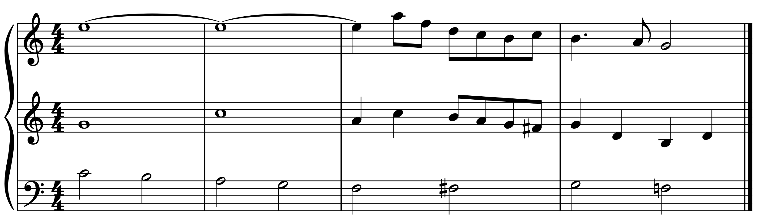
As an example, consider the following arrangement of the first four bars of Air on the G String by J. S. Bach / August Willhelmj.
Using standard MIDI numbers for notes where A4 corresponds to 69, this may be represented by the following matrix:
which we will denote A = (a_{ij}). The goal of the tuning is to translate each of these notes a_{ij} into a frequency f_{ij} \in (0, \infty). This can be done using the equal tuning by setting f_{ij} = 440 \times \tau_{\text{12-ET}}(a_{ij} - 69) for all i, j. This will result in the following:
Dynamically adaptive tuning system
To get pure intervals we instead use the following method: Assume that frequencies f_{1,1}, \ldots, f_{1,L} for the first row has been determined. Now, the frequencies for row i is defined by
This ensures that all intervals between the first and the j‘th row are just.
In order to tune the first row we can either use equal tuning, but to ensure just step intervals in the lead we instead pick a frequency for the first note, in this case f_{1,1} = 660 because the first note in the lead is A5, and define
for j > 1. The resulting arrangement with dynamically adaptive just tuning as described above sounds like this.
The tuning is dynamical, meaning that the same note played in different places in the score may be tuned to different frequencies. This may even be true for sustained notes, if the melody changes in the duration of the sustained note. As an example, the F# half-note played by the third voice in the second half of the third bar changes frequency for each 8th note duration, and is tuned as 183.33, 182.52, 183.33 and 182.52 Hz resp. in the duration of the half note.
As it is presented here, the method may be applied to a fixed score where all notes are known in advance, but it could also be used in real-time assuming the program performing the tuning has a well-defined way of determining the lead, for example the highest played note, and then use this as the base.
The code used to generate the sound clips is available on GitHub.
Literature
[1] K. Stange, C. Wick and H. Hinrichsen, “Playing Music in Just Intonation: A Dynamically Adaptive Tuning Scheme,” in Computer Music Journal, vol. 42, no. 3, pp. 47-62, Oct. 2018, doi: 10.1162/comj_a_00478.
I recently had to write a simple algorithm that computes the bit-length of an integer (the number of digits in the binary expansion of the integer) given only bitwise shifts and comparison operators. It is simple to compute the bit-length in linear time in the number of digits of the integer by computing the binary expansion and counting the number of digits, but it is also possible to do it in logarithmic running time in an upper bound for the bit-length of the integer. However, I wasn’t able to find such an algorithm described anywhere online so I share my solution here in case anyone else run into the same problem.
The idea behind the algorithm is to find the bit-length of an integer n \geq 0 using binary search with the following criterion: Find the unique m such that n \gg m = 0 but n \gg (m - 1) = 1 where \gg denotes a bitwise right shift. Note that m is the bit-length of n. Since the algorithm is a binary search, the running time is logarithmic in the maximal length of n.
Below are both a recursive and an iterative solution written in Java. They should be easy to translate to other languages.
Recursive solution
public static int bitLength(int n, int maxBitLength) {
    if (n <= 1) {
        return n;
    }
    int m = maxBitLength >> 1;
    int nPrime = n >> m;
    if (nPrime > 0) {
        return m + bitLength(nPrime, maxBitLength - m);
    }
    return bitLength(n, m);
}
Iterative solution
public static int bitLength(int n, int maxBitLength) {
    if (n <= 1) {
        return n;
    }
    int length = 1;
    while (maxBitLength > 1) {
        int m = maxBitLength >> 1;
        int nPrime = n >> m;
        if (nPrime > 0) {
            length += m;
            n = nPrime;
            maxBitLength = maxBitLength - m;
        } else {
            maxBitLength = m;
        }
    }
    return length;
}
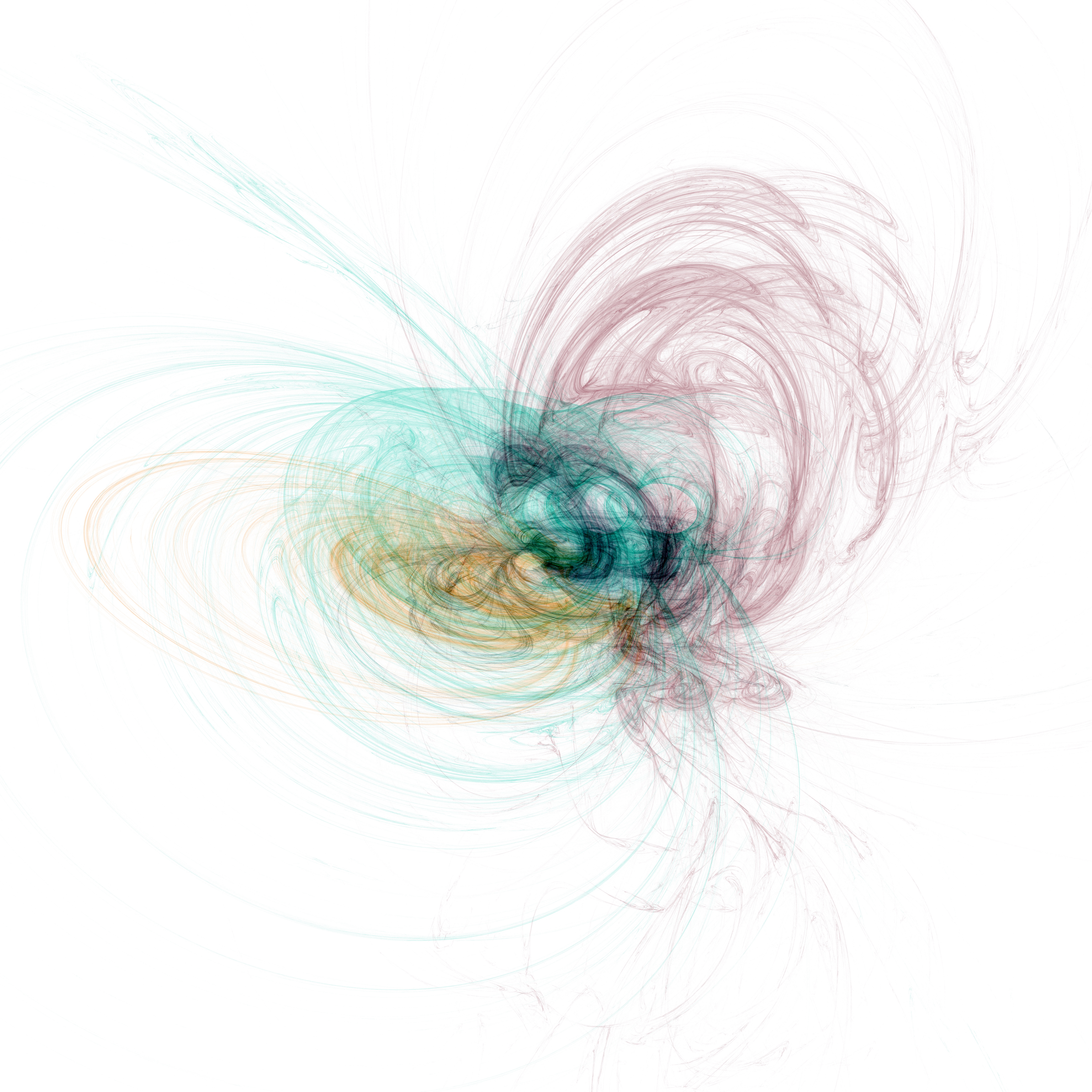
Fractal flames are a type of iterated function systems invented by Scott Draves in 1992. The fixed sets of fractal flames may be computed using the chaos game (as described in an earlier post), and the resulting histogram may be visualised as beautiful fractal-like images. If the histogram also has a dimension storing what function from the function system was used to get to a particular point, it may even be coloured.
There are a lot of software available to generate fractal flames, and I have built yet another one focussed on generating very high resolution images for printing. The image below has resolution 7087 x 7087 and been generated after about 4 hours of computation on a laptop. It is free to use under a Creative Commons BY-NC 4.0 license.
The Boids (short for “bird-like-objects”) algorithm was invented by Craig W. Reynolds in 1986 to simulate the movement of flocks of birds. One of the key insights was that a bird in a flock may be simulated using three simple rules:
Collision Avoidance: avoid collisions with nearby flockmates
Velocity Matching: attempt to match velocity with nearby flockmates
Flock Centering: attempt to stay close to nearby flockmates
Using these simple rules, a very realistically looking simulation of flocks of birds may be implemented. It is usually done in two or three dimensions, but may in principle be done in any space where direction and distance can be defined meaningfully, for example a normed vector space.
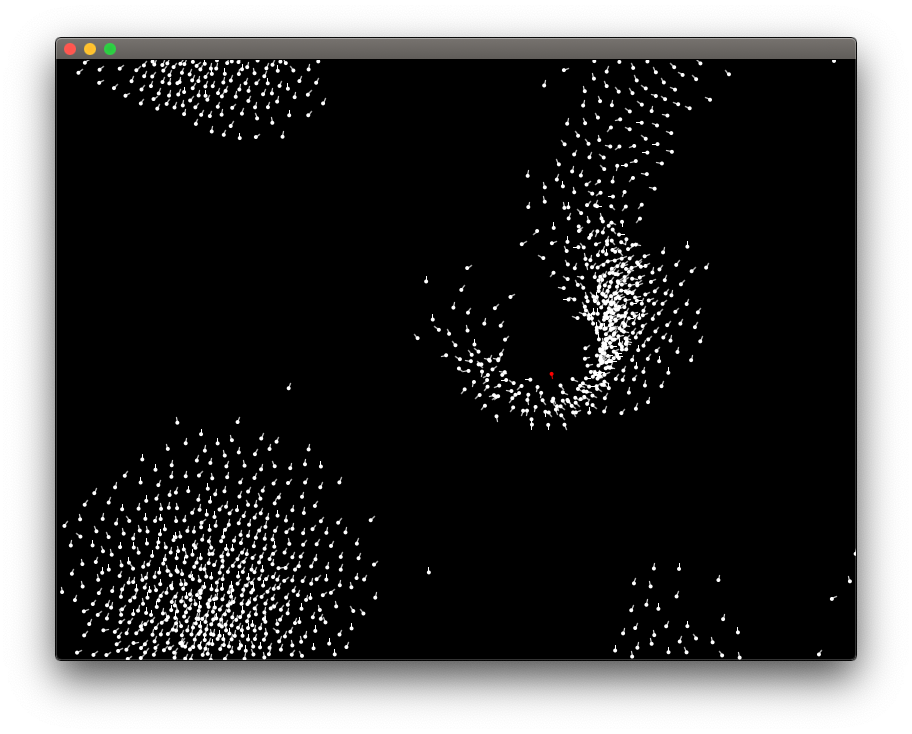
This picture is from animated simulation of a flock of birds generated using this software: https://github.com/jonas-lj/Boids. Besides the three rules from Reynolds’ paper, we have in this simulation added a red bird, a predator, which the other birds attempts to avoid.
Using the simulation to compose music
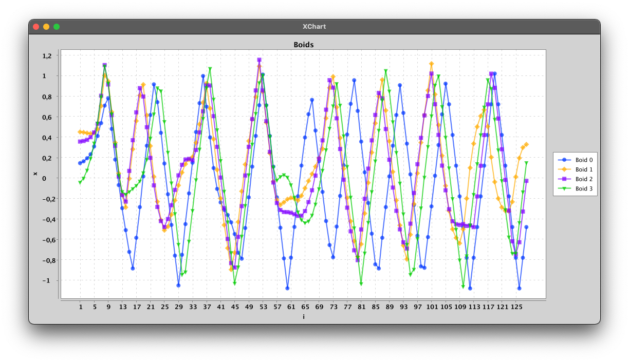
We have created a special-purpose version of the boids algorithm to compose music. In this, we limit the boids to move around in one dimension but use the same rules as in simulations in two or three dimensions. Each boid corresponds to a voice and the one-dimensional space is mapped to a set of notes in a diatonic scale. The rules are adjusted such that the collision avoidance prefers a distance of at least a third, but since there are other rules influencing the movement, and only one dimension to move around in, the boids collide often. We also add rules to keep the boids in a certain range. Left on their own, the boids tend to land in an equilibrium, so to ensure an interesting dynamic, we let one boid move randomly with its velocity changing according to a brownian motion (Boid 0 in the plot below) as well as the other rules, the boids are following. With four boids this gives a result as shown below:
A plot of a simulation of 128 iterations of four boids. The velocity of Boid 0 are changing both according to the rules but also randomly.
The voices are mapped to notes (MIDI-files) and was used in the recording all three tracks of the album “Pieces of infinity 02” by Morten Bach and Jonas Lindstrøm. The algorithm was changed slightly, for example to allow some boids to move faster than others, or to allow more boids, but the base algorithm is the same used to generate all voices for the three tracks.
The first seven bars of the four voices plotted above mapped to notes.
The Nørgård Palindrome is an ambient electronic music track released recently by Morten Bach and me. It is composed algorithmically and recorded live in studio using a lot of synthesizers. It is the second track of the album, the first being “Lorenz-6674089274190705457 (Seltsamer Attraktor)” which was described in another post.
The arpeggio-like tracks in The Nørgård Palindrome is created from an integer sequence first studied by the danish composer Per Nørgård in 1959 who called it an “infinite series”. It may be defined as
The sequence is interesting from a purely mathematical view point, which has been studied by several authors, for example by Au, Drexler-Lemire & Shallit (2017). Considering only the parity of the sequence yields the Thue-Morse sequence, which is a famous and well-studied sequence.
However, we will, as Per Nørgård, use the sequence to compose music. The sequence is most famously used in the symphony “Voyage into the Golden Screen”, where Per Nørgård mapped the first terms of the sequence to notes by picking a base note corresponding to 0 and then map an integer k to the note k semitones above the base note.
In The Nørgård Palindrome, we do the same, although we use a diatonic scale instead of a chromatic scale, and get the following notes when using a C-minor scale with 0 mapping to C:
It turns out that certain patterns are repeated throughout the sequence, although sometimes transposed, which makes the sequence very usable in music.
In the video below we play the first 144 notes slowly along while showing the progression of the corresponding sequence.
The first 144 notes of Nørgårds’ infinite series mapped to notes in a diatonic scale.
In The Nørgård Palindrome, we compute a large number of terms, allowing us to play the sequence very fast for a long time, and when done, we play the sequence backwards. This voice is played as a canon in two, and the places where the voices are in harmony or aligned emphasises the structure of the sequence.
The recurring theme is also composed from the sequence using a pentatonic scale and played slower.
The code use to generate the sequence and the MIDI-files used on the track is available on GitHub. The track is released as part of the album pieces of infinity 01 which is available on most streaming services, including Spotify and iTunes.
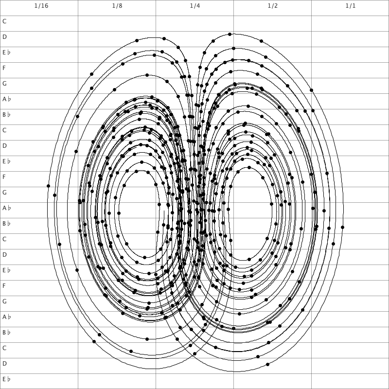
Lorenz-6674089274190705457 (Seltsamer Attraktor) is an ambient music track released by Morten Bach and me. It was composed algorithmically and recorded live in studio using a number of synthesizers. This post will describe how the track was composed.
The Lorenz system is a system of ordinary differential equations
where \sigma, \rho and \beta are positive real numbers. The system was first studied by Edward Lorenz and Helen Fetter as a simulation of atmospheric convection. It is known to behave chaotically for certain parameters since small changes in the starting point changes the future of a solution radically, an example of the so-called butterfly effect.
The differential equations above gives a formula for what direction a curve should move after it reaches a point (x,y,z) \in \mathbb{R}^3. As an example, for (1,1,1) we get the direction (0, \rho - 1, 1 - \beta).
In the composition of Lorenz-6674089274190705457 (Seltsamer Attraktor), we chose \sigma = 10, \rho = 28 and \beta = 2 and consider three curves with randomly chosen starting points. The number 6674089274190705457 is the seed of the pseudo-random number generator used to pick the starting points, so another seed would give other starting points and hence a different track.
The curves are computed numerically. Above we show an example of a curve for t \in [0, 5]. The points corresponding to a discrete subset of the three curves we get from the given seed are mapped to notes. More precisely, we pick the points where t = 0.07k for k \in \mathbb{N}.
We consider the projection of curves to the (x,z)-plane. The part of this plane where the curve resides is divided into a grid as illustrated above. If the point to be mapped to a note is in the (i,j)‘th square, the note is chosen as the j‘th note in a predefined diatonic scale (in this case C-minor) with duration 2^{-i} time-units. The resulting track is saved as a MIDI-file.
The composition of the track is visualised in a video available on YouTube. Here, all three voices are shown as separate curves along with the actual track.
The Lorenz system and this mapping into musical notes was chosen to give an interesting, and somewhat linear (musically speaking) and continuously evolving dynamic. Using this mapping, the voices composed moves both fast and slow at different times. The continuity of the curves also ensures that the movement of each voice is linear (going either up or down continuously).
The track is available on most streaming services and music platforms, eg. Spotify or iTunes. The code used to generate the tracks is available on GitHub.
Turtle graphics is a method for generating images from integer sequences using very simple rules. The drawing is done by a “turtle” which moves and draws on a plane according to some rules. At any point in time, the turtle has a position and a direction, but no other state.
For example, consider the Thue-Morse sequence defined by
Now define a turtle by the following rules. For each 0 in the sequence, the turtle rotates by \pi and for each 1, the turtle moves ahead one unit and then rotate by \frac{\pi}{3}. This gives the Koch snowflake:
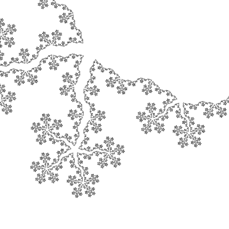
Hans Zantema has written a very nice paper on turtle graphics, including criteria for rules to ensure that the picture drawn by a turtle is either finite or self-similar. The paper also includes a number of examples, including the so-called rosettes which are defined over a binary sequence defined by the morphisms
0 \mapsto 011, 1 \mapsto 0
starting with 0. One example of a rosette is the turtle which for each 0 rotates 7 \pi / 9 and then moves, and for each 1 it rotates -2\pi / 9 and moves. This gives the following picture.
Below is a 6-minute animation of how the turtle moved while drawing the rosette.
The method can also produce more fractal-like images, like the one below which is also from Zantemas paper. Here the sequence is defined by
0 \mapsto 001100, 1 \mapsto 001101
where 0 rotates the turtle by 7\pi / 18 and 1 rotates the turtle -7 \pi / 12.
The code used to generate the pictures and video are available here.
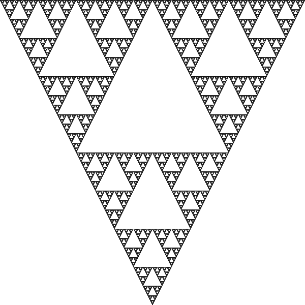
Many fractals may be described as the fixed set of an iterated function set (IFS). Perhaps most famously, the Sierpiński Triangle is such a fractal. Formally, an IFS is a set of maps on a metric space, eg. \mathbb{R}^n, which map points closer to each other.
Hutchinson proved in 1981 that an IFS has a unique compact fixed set S – a set where all points are mapped back into the set. Now, for some choices of IFS on the plane, the set S is very interesting and shows fractal properties. The Sierpiński Triangle is for example the fixed set of the following IFS:
A common way to visualise the fixed set of an IFS is by using the so-called Chaos game. Here, a point in the plane is picked at random. Then we apply one of the functions of the IFS, chosen at random, to the point. The result is another point in the plane which we again apply one of the function chosen at random on. At each step we plot the point, and we may continue for as long as we like and with as many initial points as we want.
The Sierpiński Triangle.
Another possible fractal which may be constructed as the fixed set of an IFS is the Barnsley Fern. Here the functions are (with points written as column vectors):
\begin{pmatrix} x \\ y \end{pmatrix} \mapsto \begin{pmatrix} 0 & 0 \\ 0 & 0.16 \end{pmatrix}\begin{pmatrix} x \\ y \end{pmatrix},
\begin{pmatrix} x \\ y \end{pmatrix} \mapsto \begin{pmatrix} 0.85 & 0.04 \\ -0.04 & 0.85 \end{pmatrix}\begin{pmatrix} x \\ y \end{pmatrix},
\begin{pmatrix} x \\ y \end{pmatrix} \mapsto \begin{pmatrix} 0.20 & -0.26 \\ 0.23 & 0.22 \end{pmatrix}\begin{pmatrix} x \\ y \end{pmatrix},
\begin{pmatrix} x \\ y \end{pmatrix} \mapsto \begin{pmatrix} -0.15 & 0.28 \\ 0.26 & 0.24 \end{pmatrix}\begin{pmatrix} x \\ y \end{pmatrix}.
Here, the the probability to pick the first map should be 1%, the second should be 85% and the remaining two should be 7% each. This will yield the picture below:
The Barnsley Fern.
A more complicated family of fractals representable by an IFS are the so-called fractal flames. For these fractals, the functions in their corresponding IFS’s are of the form P \circ V \circ T where P and T are affine linear transformations and V is a non-linear functions, a so-called variation.
A fractal flame.
Slowly transforming the parameters in the transformations of a fractal flame can be used to create movies.
Colouring the fractals may be done in different ways, the simplest being simply plotting each point while iterating in the chaos game. A slightly better way, which is used here, is the log-density method. Here the image to be rendered is divided into pixels, and the number of times each pixel is hit in the chaos game is saved. Now, the colour of a pixel is determined as the ratio \log n / \log m where n is the number of times the pixel was hit and m is the maximum number of times a pixel in the image has been hit.
The software used to generate the images in this post is available on GitHub.
In order to facilitate my experiments with sound synthesis, I have developed a software framework inspired by modular synthesizers, where a synthesizer consists of many connected modules, each with a very specific function. An important feature in modular synthesis is that the output of any module may be used as input in another, yielding endless possibilities in how to setup a synthesizer.
The framework is written in Java, and the core interface of the framework is the Module which has a single method which iterates the module and returns the output:
public interface Module {

  /**
   * Iterate the state of the module and return the output
   * buffer.
   *
   * @return The output of this module.
   */
  double[] getNextSamples();

}
All modules in MOSEF are instances of this interface, exploiting the polymorphism of object-oriented programming to allow the output of any module to be used as input for another. A module may take any number of inputs and give a single output.
A simple example of a Module is an Amplifier which takes a single input, and gains it by a fixed value.
public class Amplifier implements Module {

  private final double[] buffer;
  private final Module input;
  private final double gain;

  public Amplifier(MOSEFSettings settings,
                   Module input, double gain) {
    this.buffer = new double[settings.getBufferSize()];
    this.input = input;
    this.gain = gain;
  }

  @Override
  public double[] getNextSamples() {
    double[] inputBuffer = input.getNextSamples();
    for (int i = 0; i < buffer.length; i++) {
      buffer[i] = gain * inputBuffer[i];
    }
    return buffer;
  }

}
However, this amplifier can easily be changed into an amplifier where the gain is controlled by another Module. In modular synthesis this is called a voltage controlled amplifier (VCA):
public class VCA implements Module {

  private final double[] buffer;
  private final Module input, gain;

  public Amplifier(MOSEFSettings settings,
                   Module input, Module gain) {
    this.buffer = new double[settings.getBufferSize()];
    this.input = input;
    this.gain = gain;
  }

  @Override
  public double[] getNextSamples() {
    double[] inputBuffer = input.getNextSamples();
    double[] gainBuffer = gain.getNextSamples();
    for (int i = 0; i < buffer.length; i++) {
      buffer[i] = gainBuffer[i] * inputBuffer[i];
    }
    return buffer;
  }

}
Note that this a module calls the getNextSamples method on its inputs, so a more complex synthesizer will consist of many modules in a tree structure, where calling getNextSamples on the root module will call all modules the root has a input, each of which will call all modules it has as input and so on.
The framework implements a number of basic modules including
Mixers,
Oscillators and LFOs,
Delays,
Envelope generators,
Low pass filters,
Offsetters,
Glide/portamento modules,
MIDI / wav inputs,
Noise generators,
Limiters,
Arpeggiators and sequencers.
The basic modules are available through the MOSEF factory class, simplifying the code needed to design complex synthesizers. For example, pulse-width modulation synthesis where the width of a pulse wave is controlled by a low frequency sine wave may be created as follows. Here the variable m is an instance of the MOSEF factory class, and the width of the pulse wave varies between 0.3 ± 0.1 with frequency 15 Hz.