Euclidean rhythms as morphic words

Euclidean Rhythms is a method to generate rhythmic patterns which gives the most even way to distribute k onsets over n of beats with k < n. It was first discovered in 2004 by Godfried Toussaint [1] who described how these rhythms are found in music all over the world and presented an algorithm by Björklund [2] to generate the rhythms. There is also nice presentation of the math in [3]. All algorithms, including mine, relies on the Euclidean Algorithm, hence the name.

Toussaint’s paper is very interesting but I found the description of Björklunds algorithm a bit confusing. Looking at the the C code from Björklunds original paper is better, but I think it lacks some modularity and does not explain why the algorithm works.

Here, I present an algorithm to compute Euclidean Rhythms using continued fractions and morphic words. Using these concepts, the algorithm becomes very simple, and it has the added benefit that it works not only for integers n and k but for any real numbers. It is equivalent to Björklunds algorithm but is much simpler in my opinion.

Euclidean Rhythm

We represent a rhythmic pattern as a finite sequence of 0’s and 1’s where 1 is an onset and 0 is a rest. So the first half of a classic clave pattern (which can be computed as an Euclidean Rhythm with k=3 and n=8) is written as 10010010.

Generating an Euclidean Rhythm for k onsets over n of beats can be done using a cutting sequences for a straight line with slope k / n. This means that we can define the i‘th element in the sequence as

s_i = \left\lfloor \frac{(i+1)k}{n} \right\rfloor - \left\lfloor \frac{ik}{n} \right\rfloor.

This gives a geometric interpretation of Euclidean Rhythms: The goal is to distribute the onsets as evenly as possible among the beats. Note that if you use this in the example with k=3 and n=8 we get when starting from i = 0 the sequence 01001010 which is a rotation of the desired result, and we will say sequences that are equal up to rotation are equivalent.

Prerequisites

We define the rhythmic pattern as a morphic word using a family of endomorphisms:

\theta_a(x) = \begin{cases} 0^{a-1}1 & \text{if } x = 0, \\ 0^{a-1}10 & \text{if } x = 1.
\end{cases}

Note that since these are endomorphisms, they define a mapping on a word by using them on one letter at a time. So, e.g.,

\theta_2(101) = \theta_2(1) \theta_2(0) \theta_2(1) = 01001010.

Recall that a (simple) continued fraction is a representation of a real number,

a = a_0 + \frac{1}{a_1 + {\frac{1}{a_2 + \frac{1}{a_3 + \cdots}}}}

which is written a = [a_0; a_1, a_2, \ldots]. All numbers has a representation as a continued fraction, and the representation is finite if and only if it represents a rational numbers. Computing the continued fraction of a rational number is equivalent to the Euclidean Algorithm on the numerator and denominator.

The algorithm

Using these two concepts, we can define a very simple algorithm for generating an Euclidean Rhythm:

  1. Write \frac{k}{n} = [0; a_1, a_2, \ldots, a_m] as a continued fraction,
  2. Return \theta_{a_m} \circ \theta_{a_{m-1}} \circ \ldots \circ \theta_{a_1} (0).

We assume that n and k are coprime – otherwise we can reduce and simply repeat the pattern.

For the example above with k = 3 and n = 8, we get that \frac{3}{8} = [0; 2, 1, 2], so we get the Euclidean Rhythm using the morphisms in order as

0 \overset{\theta_2}{\rightarrow} 01 \overset{\theta_1}{\rightarrow} 110 \overset{\theta_2}{\rightarrow} 01001001

which is a rotation of the sequence we found above.

Non-rational patterns — a Golden rhythm

Since any number has a continued fraction representation, the above algorithm also makes sense if \frac{k}{n} is not rational. The musical interpretation of this is not as clear since it requires an infinite number of beats, but the recurrent nature of the algorithm may give a hint to what is going on.

Consider the inverse golden ratio which has continued fraction representation

\frac{-1 + \sqrt{5}}{2} = [0; 1,1,\ldots].

Since this has an infinite continued fraction expansion the above algorithm wont work directly, but if we set some limit, say m, and considers only the first m terms it gives a rational approximation which gets better as m grows. This approximation will be equal to the Euclidean Rhythm which distributes F_{m-1} onsets over F_m beats where F_m is the m‘th Fibonacci number, and will be equal to the prefix of length F_{m} of the Fibonacci word.

Source code

I have written some code in Rust which tests the equivalence of constructing Euclidean Rhythms as cutting sequences, from Björklunds Algorithm and using my algorithm.

References

[1] https://cgm.cs.mcgill.ca/~godfried/publications/banff.pdf
[2] https://www.semanticscholar.org/paper/The-Theory-of-Rep-Rate-Pattern-Generation-in-the-Bjorklund/c652d0a32895afc5d50b6527447824c31a553659
[3] https://erikdemaine.org/papers/DeepRhythms_CGTA/paper.pdf

Per Nørgaard’s Infinity Series computed iteratively

The danish composer Per Nørgaard (1932-2025) invented a serial composition method based on a sequence of integers called the “Infinity Series”. The series is most famously used in the symphony “Voyage into the Golden Screen”.

Mathematically speaking, the series is actually a sequence, and is simple to define, e.g. by

a_0 = 0 \\
a_{2n} = -a_n \\
a_{2n + 1} = a_n + 1

There are many nice articles online explaining the properties of the sequence and many ways to derive it, so we won’t go into that here. Instead we will present a way to compute the sequence iteratively based on the following equivalent formula:

a_0 = 0 \\
a_{k+1} = (-1)^{\nu_2(k)} (\nu_2(k) + 1 - a_k)

Here, \nu_2(k) is the 2-adic valuation of k which can be computed efficiently using a count trailing zeros (CTZ) function (e.g. trailing_zeros in Rust). This gives a way to compute the sequence as an iterator. In Rust, and implementation would look something like this:

pub struct NørgårdsInfinitySequence {
    previous: i64,
    index: u64,
}

impl NørgårdsInfinitySequence {
    pub fn new() -> Self {
        NørgårdsInfinitySequence {
            previous: 0,
            index: 0,
        }
    }
}

impl Iterator for NørgårdsInfinitySequence {
    type Item = i64;

    fn next(&mut self) -> Option<Self::Item> {
        if self.index > 0 {
            let v = self.index.trailing_zeros() as i64;
            self.previous = v + 1 - self.previous;
            if v.is_odd() {
                self.previous = -self.previous;
            }
        }
        self.index += 1;
        Some(self.previous)
    }
}

Dynamically Adaptive Tuning

Background

It has been known since Pythagoras that musical intervals correspond to a whole-number ratio of frequencies between the notes. The ratios for the 12 intervals in a chromatic scale are given below.

IntervalRatio
Unison1
Semitone\frac{16}{15}
Major second\frac{9}{8}
Minor third\frac{6}{5}
Major third\frac{5}{4}
Fourth\frac{4}{3}
Tritone\frac{45}{32}
Fifth\frac{3}{2}
Minor sixth\frac{8}{5}
Major sixth\frac{5}{3}
Minor seventh\frac{9}{5}
Major seventh\frac{15}{8}
Octave2

The problem is that these cannot be used as basis for for tuning an instrument because the intervals do not add up to what you would expect. As an example, you would expect that two major seconds, which is (\frac{9}{8})^2 = \frac{81}{64} would give the same ratio as a major third, but this is clearly not the case. Famously, the difference between 12 fifths and 7 octaves, which should be the same, is known as the Pythagorean comma:

\frac{(\frac{3}{2})^{12}}{2^7} \approx 1.01364.

One could fix a base note and then use the intervals from the table above to tune all keys on a piano, but because the notes are not evenly spaces, this will not allow transposition – a melody will sound different depending on what key it is played in. The most common solution to this problem is to use equal temperament which divides the octave into 12 equally sized ratios. This permits transposition but has the caveat that all intervals will only be approximately equal to their ideal ratio.

The equal temperament has been the most commonly used tuning system for centuries, but there have been some suggestions on how to improve the intonation of instruments, especially after the invention of electronic instruments. A recent example is presented in [1], where a method to compute just tuning in real-time using the method of least-squares is presented, and there is also a brief historical overview of other approaches.

Below, I present a method for optimal tunings which is very similar to the one in [1], but it is a lot simpler to understand and implement and I believe the resulting tuning is very similar. The idea behind this method is simply to use just tuning from a based on the lead/melody line. To describe it, we first need to define some formalism about tuning systems.

Tuning systems

A tuning system may be described as a strictly increasing function \tau: \mathbb{Z} \to (0, \infty) such that \tau(0) = 1. The equal tuning can, for example, be described by the relative tuning function

\tau_{\text{12-ET}}(n) = 2^{\frac{n}{12}}.

As an example of how to use this function, we first pick a base, for example that note n = 0 corresponds to A4, so it has frequency 440 Hz. The note a fifth (seven semi-tones) above then has frequency 440 Hz \times \tau_{\text{12-ET}}(7) = 659.255 Hz.

Given a base note, the just intervals in the table above defines a tuning \tau_{\text{Just}} because they define the tuning of the notes 0, \ldots, 12, and all other values may then be derived by the moving up and down in octaves, e.g. \tau_{\text{Just}}(n + 12) = 2 \tau_{\text{Just}}(n) .

We represent a score with v monophonic parts as a matrix of size v \times l with integer entries. The first row is assumed to be the leading part and l is the length of the score. The score is discretized such that a single column corresponds to the shortest note duration in the score and longer notes are represented by spanning multiple columns. This formalism cannot capture neither repeated notes nor rests, but since we are only interested in harmony, it will suffice for our purpose.

As an example, consider the following arrangement of the first four bars of Air on the G String by J. S. Bach / August Willhelmj.

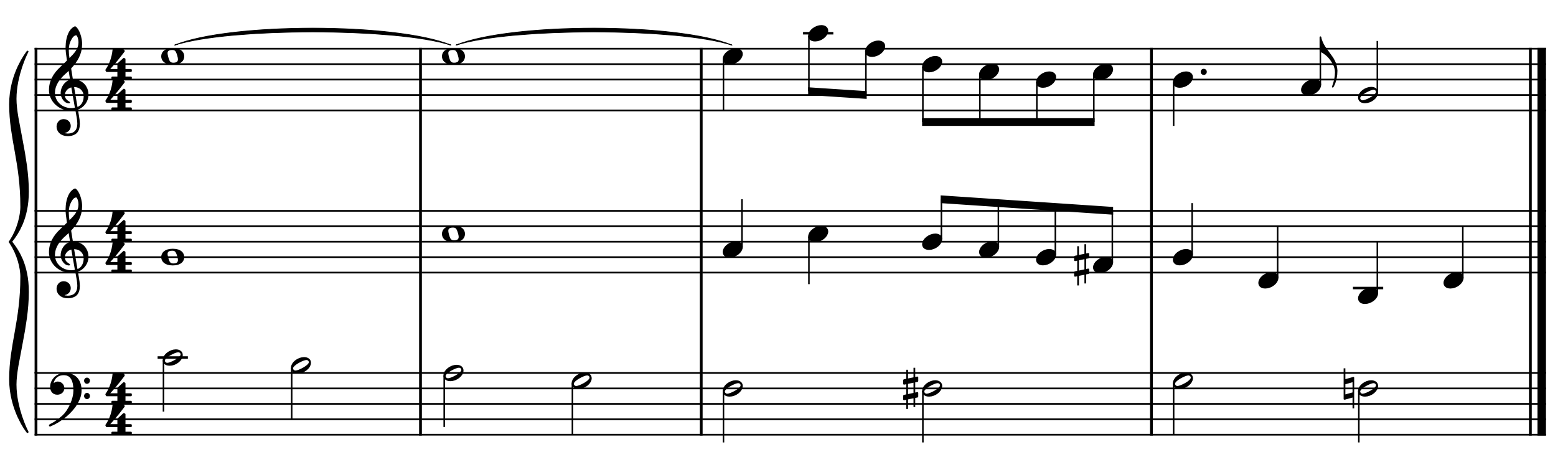
Using standard MIDI numbers for notes where A4 corresponds to 69, this may be represented by the following matrix:

\left(\begin{matrix}
76, 76, 76, 76, 76, 76, 76, 76, 76, 76, 76, 76, 76, 76, 76, 76, 76, 76, 81, 77, \cdots \\
67, 67, 67, 67, 67, 67, 67, 67, 72, 72, 72, 72, 72, 72, 72, 72, 69, 69, 72, 72, \ldots \\
60, 60, 60, 60, 59, 59, 59, 59, 57, 57, 57, 57, 55, 55, 55, 55, 53, 53, 53, 53, \ldots \\
\end{matrix}\right)

which we will denote A = (a_{ij}). The goal of the tuning is to translate each of these notes a_{ij} into a frequency f_{ij} \in (0, \infty). This can be done using the equal tuning by setting f_{ij} = 440 \times \tau_{\text{12-ET}}(a_{ij} - 69) for all i, j. This will result in the following:

Dynamically adaptive tuning system

To get pure intervals we instead use the following method: Assume that frequencies f_{1,1}, \ldots, f_{1,L} for the first row has been determined. Now, the frequencies for row i is defined by

f_{ij} = f_{1j} \tau_{\text{Just}}(a_{ij} - a_{1j}).

This ensures that all intervals between the first and the j‘th row are just.

In order to tune the first row we can either use equal tuning, but to ensure just step intervals in the lead we instead pick a frequency for the first note, in this case f_{1,1} = 660 because the first note in the lead is A5, and define

f_{1,j} = f_{1,j-1} \tau_{\text{Just}}(a_{1,j} - a_{1,j-1}).

for j > 1. The resulting arrangement with dynamically adaptive just tuning as described above sounds like this.

The tuning is dynamical, meaning that the same note played in different places in the score may be tuned to different frequencies. This may even be true for sustained notes, if the melody changes in the duration of the sustained note. As an example, the F# half-note played by the third voice in the second half of the third bar changes frequency for each 8th note duration, and is tuned as 183.33, 182.52, 183.33 and 182.52 Hz resp. in the duration of the half note.

As it is presented here, the method may be applied to a fixed score where all notes are known in advance, but it could also be used in real-time assuming the program performing the tuning has a well-defined way of determining the lead, for example the highest played note, and then use this as the base.

The code used to generate the sound clips is available on GitHub.

Literature

[1] K. Stange, C. Wick and H. Hinrichsen, “Playing Music in Just Intonation: A Dynamically Adaptive Tuning Scheme,” in Computer Music Journal, vol. 42, no. 3, pp. 47-62, Oct. 2018, doi: 10.1162/comj_a_00478.