In an earlier post I described a way to sample a uniformly random derangement, a permutation with no fixed points, in linear time and without any big-integer arithmetic. Since then I have created samplers for a couple of similar objects, like involutions, which are permutations equal to their own inverse, and perfect matchings, which are involutions with no fixed points. Writing the third one I noticed that they are all the same algorithm.
The thing they have in common is the cycle structure. A derangement is a permutation whose cycles all have length \geq 2, an involution has cycles of length \leq 2 and a matching has cycles of length exactly 2. In every case we pick a set S of permitted cycle lengths and ask for a uniformly random permutation built from those alone.
Counting such permutations is a single recurrence. Let a_n be the number of permutations of n elements whose cycle lengths all lie in S. The largest element must sit in a cycle of some length k \in S. There are (n-1)(n-2)\cdots(n-k+1) ways to line up its k-1 cycle-mates in order, and the remaining elements form a smaller instance of the same problem, so
To sample a uniformly random permutation of the given type, repeatedly take the largest remaining element and give it a cycle of length k with probability proportional to the k-th term above, then draw its k-1 partners uniformly at random. Each valid permutation then turns up with probability exactly \frac{1}{a_n}.
One problem is that a_n grows like n!, so forming those weights directly overflows almost immediately. We sidestep this by never building the numbers at all. The probabilities are computed iteratively, so no big integers are needed however large n gets.
Recall that a derangement is a permutation without fixed points. The problem of computing the number of such derangements on a set of size n is also known as the subfactorial, denoted !n and was first solved by Pierre Raymond de Montmort in 1713. It is now known that
!n = \left\lfloor \frac{n!}{e} \right\rfloor
which is the source of the joke about that the probability that none of n drunk mathematicians get their own coat after a dinner party is 1/e.
A simple way to sample a random derangement is use rejection sampling and sample random permutations until you get a derangement, e.g. using the Fisher-Yates shuffle. So on average, e samplings will be sufficient to get a derangement.
A nicer way to do this, which avoids the rejection sampling, is presented in “Generating Random Derangements” by Martínez, Panholzer and Prodinger. This method has complexity similar to that of the Fisher-Yates shuffle and is simple to implement. Here, I present a slight variation of Martínez et.al’s algorithm with two improvements:
It avoids a rejection sampling on the index to swap with. I found this a bit annoying since one of the reasons for not using Fisher-Yates is to avoid rejection sampling.
By using a different data structure for the marked elements, I avoid one of the nested if statements.
The complexity and performance should be about the same as the original algorithm but it is slightly more elegant in my opinion.
The code looks as follows in Rust:
/// The probabilities that, with `u + 1` elements left to place, the current one closes a 2-cycle rather than extending into a longer cycle.
pub fn two_cycle_probabilities() -> impl Iterator<Item = f64> {
successors(Some((0usize, 0.0f64)), |&(mut u, prev)| {
u += 1;
Some((u, (1.0 - prev) / (u as f64 - prev)))
})
.map(|(_, p)| p)
}
pub fn sample_derangement(n: usize) -> Vec<usize> {
if n == 0 {
return Vec::new();
} else if n == 1 {
panic!("no derangement exists for n = 1");
}
let mut rng = rand::rng();
let two_cycle_prob = two_cycle_probabilities().take(n).collect::<Vec<f64>>();
let mut permutation = (0..n).collect::<Vec<usize>>();
let mut unmarked = (0..n).collect::<Vec<usize>>();
while unmarked.len() > 1 {
let i = unmarked.pop().unwrap();
let j = rng.random_range(..unmarked.len());
permutation.swap(i, unmarked[j]);
if rng.random_bool(two_cycle_prob[unmarked.len()]) {
unmarked.swap_remove(j);
}
}
permutation
}
I recently ran into a situation where I needed a fast way to evaluate a polynomial on inputs 1,...,n where n. It turns out that there is a way of doing this quicker than just computing the evaluation using something like Horner’s method on each input, assuming that n is sufficiently larger than the degree of the polynomial. As with many other ingenious algorithms, this one can be found in Donald Knuth’s “The Art of Computer Programming”, where it’s mentioned briefly in section 4.6.4 and left as an exercise, and it gives something more general, namely a way to compute evaluations on points in arithmetic progression. Here I give some more details about the algorithm and provide an implementation in Rust.
Let f(x) = f_0 + f_1x + \cdots + f_d x^d be a polynomial in some ring and let x_0 and h define an arithmetic progression, x_0, x_0 + h, x_0 + 2h, \ldots. There is a pre-computation step before we can get to the actual evaluation: First we compute the evaluations of the first d+1 elements of the arithmetic progression:
y_j = f(x_0 + jh), \quad j = 0,\ldots,d.
Since this gives us the first d+1 evaluations, this proves that the method is not quicker if we need fewer points than d+1. To complete the pre-processing, we let for all k=1,\ldots,d and j=d,\ldots,k (going down)
y_j = y_j - y_{j-1}.
Now, y_0 holds the evaluation of the first value in the arithmetic progression, i.e. f(x_0), and we can implement the evaluation as an iterator. To get the next evaluation, let for j = 0,\ldots, d-1,
y_j = y_j + y_{j+1},\qquad (1)
and yield y_0 as the next evaluation. Notice that in this step, an evaluation can be computed with d additions where a naive evaluation using Horner’s method requires d additions andd multiplications.
The correctness rests on the forward difference \Delta f(x) = f(x+h) - f(x). Since \Delta lowers degree by one, \Delta^{d+1} f = 0. After preprocessing, the subtractions y_j \gets y_j - y_{j-1} leave y_j = \Delta^j f(x_0) for j = 0,\ldots,d.
The loop maintains the invariant y_j = \Delta^j f(x_0 + ih). It holds at i=0, and the update y_j \gets y_j + y_{j+1} advances it by one step, since \Delta^j f(x+h) = \Delta^j f(x) + \Delta^{j+1} f(x). Here, y_d is constant and untouched. Thus y_0 = f(x_0 + ih) at each yield, using d additions and no multiplications.
There are a few optimisations that can be implemented for this algorithm:
Since the first d+1 evaluations are computed in the preprocessing, we can store these and yield them directly. This is a very small optimisation since the iteration step (1) has to be computed anyway, and it gives larger state for the iterator.
Notice that for a single iteration, y_0 only depends on y_0 and y_1, so for the last iterations of this iterator, some of the steps in (1) can be skipped.
The algorithm implemented in Rust is available on GitHub.
Most Lego instructions put bricks aligned with the grid, but a few of them uses bricks at angles, for example the Corner Garage. If we look at a Lego board as a coordinate system, and assume that the brick we want to put at an angle has one end in (0,0), then it is possible to end it at a stud at (a,b) if there is an integer c such that a^2 + b^2 = c^2. This is known as a Pythagorean triple, and it is known that there are infinitely many of these. The smallest one, which can also be used in Lego is (3,4,5), so a 6 stud piece can be put at an angle from a stud to the stud 4 studs to the right and 3 studs above. Note that we need a 6 stud piece to cover a distance of 5.
Near Pythagorean triples
There are only a few small Pythagorean triples usable in Lego construction, where the longest brick is 16 studs long. However, in the Corner Garage mentioned earlier, they use a triple (12, 12, 17) to produce a 45° angle, but this is not a Pythagorean triple since \sqrt{12^2 + 12^2} = 16.9706 \neq 17. The error (distance to nearest stud) for this Lego approved triple is ~0.03, so we use this as an upper bound on the triples computed here.
We may extend the list of triples further because there are Lego pieces which allow us to put a brick half-way between studs, so we do not need to restrict ourselves to integers but may include half-integers too. If we restrict the coordinates to be at most 15 units long, there are 71 triples. Sorted by angle they are:
Note that only angles up to 45 degrees are included here, since larger angles can be constructed from symmetry. Below are pictures of two examples of the triples (7.5, 4, 8.5) (left) and (6, 2.5, 6.5) .
Vertical angles
The above example is for putting bricks horizontally on a plate. However, some bricks, like Lego Technic bricks or the “light holder” bricks, allows you to build vertical angles as well, because you can put a brick on the side of it.
The height of a brick and the with of one stud is, however, not equal, so the Pythagorean triples have to be computed differently. We still allow the horizontal axis to be integers and half-integers, as above, but for the vertical axis, we use the unit size of one place. If you’ve ever built with Legos, you probably know that three plates equals one brick, but it is also true that that five plates equal two studs. So the if we keep using one horizontal stud as a unit, the vertical coordinate must be a multiple of \frac{2}{5}. This gives the following list of 33 near Pythagorean triples:
Below is a picture of a usage of the triples (6, 3.6, 7) and (7.5, 2.8, 8). Recall that 0.4 on the vertical axis corresponds to one plate and 1.2 is the full height of a brick.
Source code
The source code used to compute the triples is available here.
It has been known since Pythagoras that musical intervals correspond to a whole-number ratio of frequencies between the notes. The ratios for the 12 intervals in a chromatic scale are given below.
Interval
Ratio
Unison
1
Semitone
\frac{16}{15}
Major second
\frac{9}{8}
Minor third
\frac{6}{5}
Major third
\frac{5}{4}
Fourth
\frac{4}{3}
Tritone
\frac{45}{32}
Fifth
\frac{3}{2}
Minor sixth
\frac{8}{5}
Major sixth
\frac{5}{3}
Minor seventh
\frac{9}{5}
Major seventh
\frac{15}{8}
Octave
2
The problem is that these cannot be used as basis for for tuning an instrument because the intervals do not add up to what you would expect. As an example, you would expect that two major seconds, which is (\frac{9}{8})^2 = \frac{81}{64} would give the same ratio as a major third, but this is clearly not the case. Famously, the difference between 12 fifths and 7 octaves, which should be the same, is known as the Pythagorean comma:
\frac{(\frac{3}{2})^{12}}{2^7} \approx 1.01364.
One could fix a base note and then use the intervals from the table above to tune all keys on a piano, but because the notes are not evenly spaces, this will not allow transposition – a melody will sound different depending on what key it is played in. The most common solution to this problem is to use equal temperament which divides the octave into 12 equally sized ratios. This permits transposition but has the caveat that all intervals will only be approximately equal to their ideal ratio.
The equal temperament has been the most commonly used tuning system for centuries, but there have been some suggestions on how to improve the intonation of instruments, especially after the invention of electronic instruments. A recent example is presented in [1], where a method to compute just tuning in real-time using the method of least-squares is presented, and there is also a brief historical overview of other approaches.
Below, I present a method for optimal tunings which is very similar to the one in [1], but it is a lot simpler to understand and implement and I believe the resulting tuning is very similar. The idea behind this method is simply to use just tuning from a based on the lead/melody line. To describe it, we first need to define some formalism about tuning systems.
Tuning systems
A tuning system may be described as a strictly increasing function \tau: \mathbb{Z} \to (0, \infty) such that \tau(0) = 1. The equal tuning can, for example, be described by the relative tuning function
\tau_{\text{12-ET}}(n) = 2^{\frac{n}{12}}.
As an example of how to use this function, we first pick a base, for example that note n = 0 corresponds to A4, so it has frequency 440 Hz. The note a fifth (seven semi-tones) above then has frequency 440 Hz \times \tau_{\text{12-ET}}(7) = 659.255 Hz.
Given a base note, the just intervals in the table above defines a tuning \tau_{\text{Just}} because they define the tuning of the notes 0, \ldots, 12, and all other values may then be derived by the moving up and down in octaves, e.g. \tau_{\text{Just}}(n + 12) = 2 \tau_{\text{Just}}(n) .
We represent a score with v monophonic parts as a matrix of size v \times l with integer entries. The first row is assumed to be the leading part and l is the length of the score. The score is discretized such that a single column corresponds to the shortest note duration in the score and longer notes are represented by spanning multiple columns. This formalism cannot capture neither repeated notes nor rests, but since we are only interested in harmony, it will suffice for our purpose.
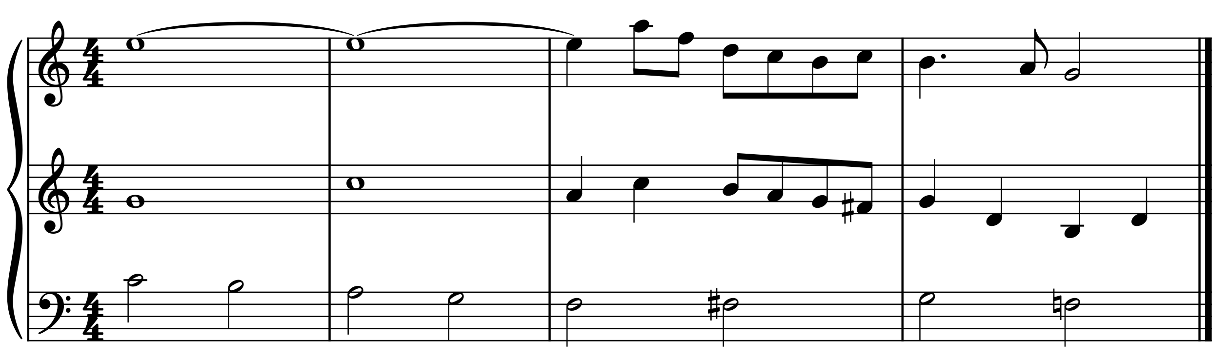
As an example, consider the following arrangement of the first four bars of Air on the G String by J. S. Bach / August Willhelmj.
Using standard MIDI numbers for notes where A4 corresponds to 69, this may be represented by the following matrix:
which we will denote A = (a_{ij}). The goal of the tuning is to translate each of these notes a_{ij} into a frequency f_{ij} \in (0, \infty). This can be done using the equal tuning by setting f_{ij} = 440 \times \tau_{\text{12-ET}}(a_{ij} - 69) for all i, j. This will result in the following:
Dynamically adaptive tuning system
To get pure intervals we instead use the following method: Assume that frequencies f_{1,1}, \ldots, f_{1,L} for the first row has been determined. Now, the frequencies for row i is defined by
This ensures that all intervals between the first and the j‘th row are just.
In order to tune the first row we can either use equal tuning, but to ensure just step intervals in the lead we instead pick a frequency for the first note, in this case f_{1,1} = 660 because the first note in the lead is A5, and define
for j > 1. The resulting arrangement with dynamically adaptive just tuning as described above sounds like this.
The tuning is dynamical, meaning that the same note played in different places in the score may be tuned to different frequencies. This may even be true for sustained notes, if the melody changes in the duration of the sustained note. As an example, the F# half-note played by the third voice in the second half of the third bar changes frequency for each 8th note duration, and is tuned as 183.33, 182.52, 183.33 and 182.52 Hz resp. in the duration of the half note.
As it is presented here, the method may be applied to a fixed score where all notes are known in advance, but it could also be used in real-time assuming the program performing the tuning has a well-defined way of determining the lead, for example the highest played note, and then use this as the base.
The code used to generate the sound clips is available on GitHub.
Literature
[1] K. Stange, C. Wick and H. Hinrichsen, “Playing Music in Just Intonation: A Dynamically Adaptive Tuning Scheme,” in Computer Music Journal, vol. 42, no. 3, pp. 47-62, Oct. 2018, doi: 10.1162/comj_a_00478.
Turtle graphics is a method for generating images from integer sequences using very simple rules. The drawing is done by a “turtle” which moves and draws on a plane according to some rules. At any point in time, the turtle has a position and a direction, but no other state.
For example, consider the Thue-Morse sequence defined by
Now define a turtle by the following rules. For each 0 in the sequence, the turtle rotates by \pi and for each 1, the turtle moves ahead one unit and then rotate by \frac{\pi}{3}. This gives the Koch snowflake:
Hans Zantema has written a very nice paper on turtle graphics, including criteria for rules to ensure that the picture drawn by a turtle is either finite or self-similar. The paper also includes a number of examples, including the so-called rosettes which are defined over a binary sequence defined by the morphisms
0 \mapsto 011, 1 \mapsto 0
starting with 0. One example of a rosette is the turtle which for each 0 rotates 7 \pi / 9 and then moves, and for each 1 it rotates -2\pi / 9 and moves. This gives the following picture.
Below is a 6-minute animation of how the turtle moved while drawing the rosette.
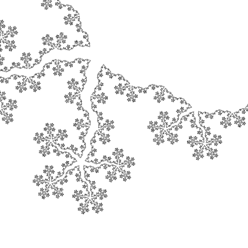
The method can also produce more fractal-like images, like the one below which is also from Zantemas paper. Here the sequence is defined by
0 \mapsto 001100, 1 \mapsto 001101
where 0 rotates the turtle by 7\pi / 18 and 1 rotates the turtle -7 \pi / 12.
The code used to generate the pictures and video are available here.