Using the “Boids” algorithm to compose music

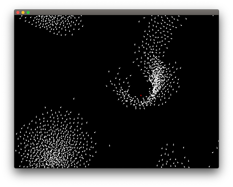
Simulating flocks of birds

The Boids (short for “bird-like-objects”) algorithm was invented by Craig W. Reynolds in 1986 to simulate the movement of flocks of birds. One of the key insights was that a bird in a flock may be simulated using three simple rules:

  1. Collision Avoidance: avoid collisions with nearby flockmates
  2. Velocity Matching: attempt to match velocity with nearby flockmates
  3. Flock Centering: attempt to stay close to nearby flockmates

Using these simple rules, a very realistically looking simulation of flocks of birds may be implemented. It is usually done in two or three dimensions, but may in principle be done in any space where direction and distance can be defined meaningfully, for example a normed vector space.

This picture is from animated simulation of a flock of birds generated using this software: https://github.com/jonas-lj/Boids. Besides the three rules from Reynolds’ paper, we have in this simulation added a red bird, a predator, which the other birds attempts to avoid.

Using the simulation to compose music

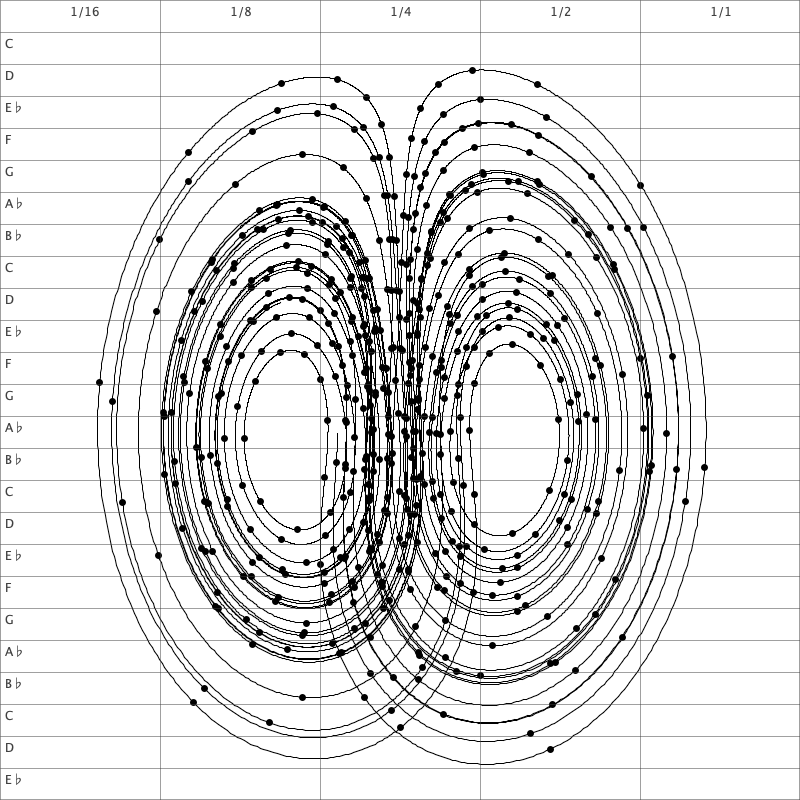
We have created a special-purpose version of the boids algorithm to compose music. In this, we limit the boids to move around in one dimension but use the same rules as in simulations in two or three dimensions. Each boid corresponds to a voice and the one-dimensional space is mapped to a set of notes in a diatonic scale. The rules are adjusted such that the collision avoidance prefers a distance of at least a third, but since there are other rules influencing the movement, and only one dimension to move around in, the boids collide often. We also add rules to keep the boids in a certain range. Left on their own, the boids tend to land in an equilibrium, so to ensure an interesting dynamic, we let one boid move randomly with its velocity changing according to a brownian motion (Boid 0 in the plot below) as well as the other rules, the boids are following. With four boids this gives a result as shown below:

A plot of a simulation of 128 iterations of four boids. The velocity of Boid 0 are changing both according to the rules but also randomly.

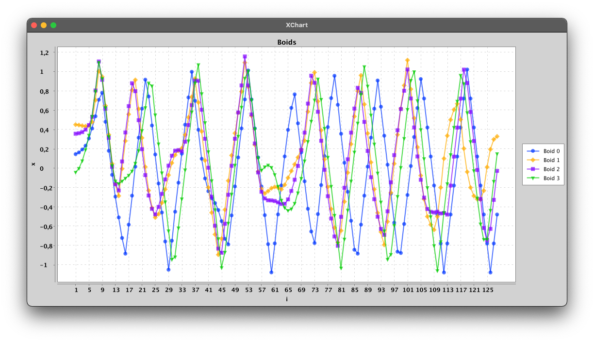
The voices are mapped to notes (MIDI-files) and was used in the recording all three tracks of the album “Pieces of infinity 02” by Morten Bach and Jonas Lindstrøm. The algorithm was changed slightly, for example to allow some boids to move faster than others, or to allow more boids, but the base algorithm is the same used to generate all voices for the three tracks.

The first seven bars of the four voices plotted above mapped to notes.

References

Reynolds, Craig (1987): Flocks, herds and schools: A distributed behavioural model. SIGGRAPH ’87: Proceedings of the 14th Annual Conference on Computer Graphics and Interactive Techniques, https://team.inria.fr/imagine/files/2014/10/flocks-hers-and-schools.pdf

Lindstrøm, Jonas (2022): boid-composer, https://github.com/jonas-lj/boid-composer

On the creation of “The Nørgård Palindrome”

The Nørgård Palindrome is an ambient electronic music track released recently by Morten Bach and me. It is composed algorithmically and recorded live in studio using a lot of synthesizers. It is the second track of the album, the first being “Lorenz-6674089274190705457 (Seltsamer Attraktor)” which was described in another post.

The arpeggio-like tracks in The Nørgård Palindrome is created from an integer sequence first studied by the danish composer Per Nørgård in 1959 who called it an “infinite series”. It may be defined as

\begin{aligned}
a_0 &= 0, \\
a_{2n} &= -a_n, \\
a_{2n + 1} &= a_n + 1.
\end{aligned}

The first terms of the sequence are

0, 1, -1, 2, 1, 0, -2, 3, -1, 2, 0, 1, 2, -1, -3, 4, 1, 0, \ldots

The sequence is interesting from a purely mathematical view point, which has been studied by several authors, for example by Au, Drexler-Lemire & Shallit (2017). Considering only the parity of the sequence yields the Thue-Morse sequence, which is a famous and well-studied sequence.

However, we will, as Per Nørgård, use the sequence to compose music. The sequence is most famously used in the symphony “Voyage into the Golden Screen”, where Per Nørgård mapped the first terms of the sequence to notes by picking a base note corresponding to 0 and then map an integer k to the note k semitones above the base note.

In The Nørgård Palindrome, we do the same, although we use a diatonic scale instead of a chromatic scale, and get the following notes when using a C-minor scale with 0 mapping to C:

It turns out that certain patterns are repeated throughout the sequence, although sometimes transposed, which makes the sequence very usable in music.

In the video below we play the first 144 notes slowly along while showing the progression of the corresponding sequence.

The first 144 notes of Nørgårds’ infinite series mapped to notes in a diatonic scale.

In The Nørgård Palindrome, we compute a large number of terms, allowing us to play the sequence very fast for a long time, and when done, we play the sequence backwards. This voice is played as a canon in two, and the places where the voices are in harmony or aligned emphasises the structure of the sequence.

The recurring theme is also composed from the sequence using a pentatonic scale and played slower.

The code use to generate the sequence and the MIDI-files used on the track is available on GitHub. The track is released as part of the album pieces of infinity 01 which is available on most streaming services, including Spotify and iTunes.

On the creation of “Lorenz-6674089274190705457 (Seltsamer Attraktor)”

Lorenz-6674089274190705457 (Seltsamer Attraktor) is an ambient music track released by Morten Bach and me. It was composed algorithmically and recorded live in studio using a number of synthesizers. This post will describe how the track was composed.

The Lorenz system is a system of ordinary differential equations

\begin{aligned}
\frac{\mathrm{d}x}{\mathrm{d}t} &= \sigma(y - x), \\
\frac{\mathrm{d}y}{\mathrm{d}t} &= x(\rho - z) - y, \\
\frac{\mathrm{d}z}{\mathrm{d}t} &= xy - \beta z.
\end{aligned}

where \sigma, \rho and \beta are positive real numbers. The system was first studied by Edward Lorenz and Helen Fetter as a simulation of atmospheric convection. It is known to behave chaotically for certain parameters since small changes in the starting point changes the future of a solution radically, an example of the so-called butterfly effect.

The differential equations above gives a formula for what direction a curve should move after it reaches a point (x,y,z) \in \mathbb{R}^3. As an example, for (1,1,1) we get the direction (0, \rho - 1, 1 - \beta).

In the composition of Lorenz-6674089274190705457 (Seltsamer Attraktor), we chose \sigma = 10, \rho = 28 and \beta = 2 and consider three curves with randomly chosen starting points. The number 6674089274190705457 is the seed of the pseudo-random number generator used to pick the starting points, so another seed would give other starting points and hence a different track.

The curves are computed numerically. Above we show an example of a curve for t \in [0, 5]. The points corresponding to a discrete subset of the three curves we get from the given seed are mapped to notes. More precisely, we pick the points where t = 0.07k for k \in \mathbb{N}.

We consider the projection of curves to the (x,z)-plane. The part of this plane where the curve resides is divided into a grid as illustrated above. If the point to be mapped to a note is in the (i,j)‘th square, the note is chosen as the j‘th note in a predefined diatonic scale (in this case C-minor) with duration 2^{-i} time-units. The resulting track is saved as a MIDI-file.

The composition of the track is visualised in a video available on YouTube. Here, all three voices are shown as separate curves along with the actual track.

The Lorenz system and this mapping into musical notes was chosen to give an interesting, and somewhat linear (musically speaking) and continuously evolving dynamic. Using this mapping, the voices composed moves both fast and slow at different times. The continuity of the curves also ensures that the movement of each voice is linear (going either up or down continuously).

The track is available on most streaming services and music platforms, eg. Spotify or iTunes. The code used to generate the tracks is available on GitHub.

MOSEF – a MOdular Synthesizer Framework for Java

In order to facilitate my experiments with sound synthesis, I have developed a software framework inspired by modular synthesizers, where a synthesizer consists of many connected modules, each with a very specific function. An important feature in modular synthesis is that the output of any module may be used as input in another, yielding endless possibilities in how to setup a synthesizer.

The framework is written in Java, and the core interface of the framework is the Module which has a single method which iterates the module and returns the output:

public interface Module {

  /**
   * Iterate the state of the module and return the output
   * buffer.
   * 
   * @return The output of this module.
   */
  double[] getNextSamples();

}

All modules in MOSEF are instances of this interface, exploiting the polymorphism of object-oriented programming to allow the output of any module to be used as input for another. A module may take any number of inputs and give a single output.

A simple example of a Module is an Amplifier which takes a single input, and gains it by a fixed value.

public class Amplifier implements Module {

  private final double[] buffer;
  private final Module input;
  private final double gain;

  public Amplifier(MOSEFSettings settings, 
                   Module input, double gain) {
    this.buffer = new double[settings.getBufferSize()];
    this.input = input;
    this.gain = gain;
  }

  @Override
  public double[] getNextSamples() {
    double[] inputBuffer = input.getNextSamples();
    for (int i = 0; i < buffer.length; i++) {
      buffer[i] = gain * inputBuffer[i];
    }
    return buffer;
  }

}

However, this amplifier can easily be changed into an amplifier where the gain is controlled by another Module. In modular synthesis this is called a voltage controlled amplifier (VCA):

public class VCA implements Module {

  private final double[] buffer;
  private final Module input, gain;

  public Amplifier(MOSEFSettings settings, 
                   Module input, Module gain) {
    this.buffer = new double[settings.getBufferSize()];
    this.input = input;
    this.gain = gain;
  }

  @Override
  public double[] getNextSamples() {
    double[] inputBuffer = input.getNextSamples();
    double[] gainBuffer = gain.getNextSamples();
    for (int i = 0; i < buffer.length; i++) {
      buffer[i] = gainBuffer[i] * inputBuffer[i];
    }
    return buffer;
  }

}

Note that this a module calls the getNextSamples method on its inputs, so a more complex synthesizer will consist of many modules in a tree structure, where calling getNextSamples on the root module will call all modules the root has a input, each of which will call all modules it has as input and so on.

The framework implements a number of basic modules including

  • Mixers,
  • Oscillators and LFOs,
  • Delays,
  • Envelope generators,
  • Low pass filters,
  • Offsetters,
  • Glide/portamento modules,
  • MIDI / wav inputs,
  • Noise generators,
  • Limiters,
  • Arpeggiators and sequencers.

The basic modules are available through the MOSEF factory class, simplifying the code needed to design complex synthesizers. For example, pulse-width modulation synthesis where the width of a pulse wave is controlled by a low frequency sine wave may be created as follows. Here the variable m is an instance of the MOSEF factory class, and the width of the pulse wave varies between 0.3 ± 0.1 with frequency 15 Hz.

Module modulator = m.offset(m.sine(15.0), 0.3, 0.1);
Module oscillator = m.pulse(in, modulator);

The framework is available on GitHub as well as some examples on how to use the framework.

Algorithmic composition with Langton’s Ant

Langton’s Ant is a simulation in two dimensions which has been proven to be a universal Turing machine – so it can in principal be used to compute anything computable by a computer.

The simulation consists of an infinite board of squares which can be either white or black. Now, an ant walks around the board. If the ant lands on a white square, it turns right, flips the color of the square and moves forward. one square If the square is black, the ant turns left, flips the color of the square and moves forward one square.

When visualised, the behaviour of this system changes over time from structured and simple to more chaotic. However, the system is completely deterministic, determined only by the starting state.

In the video above, a simulation with two ants runs over 500 steps and every time a square flips from black to white a note is played. The note to be played is determined as follows:

  • The board is divided into 7×7 sub-boards.
  • These squares are enumerated from the bottom left from 0 to 48.
  • When a square is flipped from black to white, the number assigned to the square determines the note as the number of semitones above A1.

Seven is chosen as the width of the sub-squares because it is the number of semitones in a fifth, so the ants moves either chromatically (horizontally) or in fifths (vertically). In the beginning, they are moving independently and very structured, but when their paths meet, a more complex, chaotic behaviour emerges.

DIY preamp for Leslie 760

I have recently bought a used Leslie 760 amplifier, but unfortunately it came without the pedal used to change the speed of the rotator and which also acts as preamp. A used pedal and the necessary cables is priced at about €400 so I decided to build one myself.

Luckily, some nice people has posted scanned versions of the old manuals for Leslie amps and put them online: http://www.captain-foldback.com/Leslie_sub/leslie_manuals.htm.

The amplifier does not have a normal jack-plug for connection with an instrument but has instead a 9-pole plug. At first glance, this seems a bit confusing, but it is quite simple: Pole 1 is ground and pole 2 is sound input. The rotator is activated by grounding pole 6 (slow) or pole 7 (fast).

With this information it was easy to build everything I needed: I built a small box with room for two jack plugs to be put on the amp. The first plug is mono for instrument connection, and is attached to pole 1 and 2. The other plug is for stereo which is connected to pole 6 and 7 (and ground). At the other end of this stereo cable I attached a switch pedal with two buttons: One for switching between grounding the two poles of the stereo jack and another for switching the connection on/off. I got everything for about €25 on musik-ding.de.

I still needed a preamp and found one by the brand ‘Art’ at 4Sound.dk for €35, so for about 60€ I got everything I needed to run the amp.

You are more than welcome to write me at mail@jonaslindstrom.dk if you have any questions.