Introduction

I have recently read The Expected Goals Philosophy by James Tippett, where the idea behind “Expected goals” is explained very well. In The Expected Goals Philosophy, the probability that a given team will win based on their expected goals is computed by simulating the game many times, but it can actually be computed analytically which I will do here.

Also in The Expected Goals Philosophy, a phenomenon where a team creating a few good chances will win against a team creating many smaller chances even though the expected number of goals is exactly the same, is introduced and explained. Here I will give a different, and perhaps more rigorous explanation than the one given in the book to this curious phenomenon.

The distribution of xG

First, lets sum up the concept of expected goals: Given the shots a football team has during a match, each with some probability of ending up as a goal, the expected goals (xG) is the expected value of the total number of goals which equals the sum of the probabilities of each shot ending up in goal.

A shot with probability p of ending up in goal can be considered to be a Bernoulli random variable, so the expected goals of a team is the sum of many Bernoulli random variables, one for each shot. It follows that the expected goals of a team has a Poisson binomial distribution.

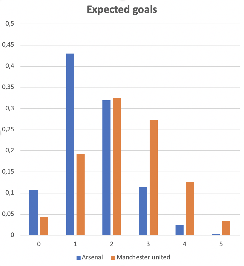
Consider the following example from The Expected Goals Philosophy. In 2019 Arsenal played Manchester United. The shots taken by each team and their estimated probabilities of ending up in goal are listed below:

Arsenal shots: (0.02, 0.02, 0.03, 0.04, 0.04, 0.05, 0.06, 0.07, 0.09, 0.10, 0.12, 0.13, 0.76)

Manchester United shots: (0.01, 0.02, 0.02, 0.02, 0.03, 0.05, 0.05, 0.05, 0.06, 0.22, 0.30, 0.43, 0.48, 0.63)

The expected value of a Poisson binomial distribution is the sum of the probabilities of each experiment (shot in this case), so calculating the expected goals for each team is simple: Arsenal has xG = 1.53 and Manchester United has xG = 2.37. But to consider the distribution of who will win the game, we need to consider the probability mass function of the expected goals which, as we saw, has a Poisson binomial distrbution.

The pmf of a Poisson binomial distributed random variable X with n parameters p_1, \ldots, p_n (shots with estimated xG’s in this case) may be calculated as follows: The probability that exactly k shots succeeds is equal to the sum of all possible combinations of k shots succeeding and the remaining n-k shots missed, e.g.

P(X = k) = \sum_{A \in F_{k,n}} \prod_{i \in A} p_i \prod_{j \in F_{k,n} \setminus A} (1-p_j).

Here F_{k,n} is the set of all subsets of size k of \{1,\ldots,n\}. The pmf in this form is cumbersome to compute when the number of parameters (in this case the number of shots) increases. But luckily there are smarter ways to compute them, eg. a recursive method which is used in the code used to compute the actual distribution:

Now computing the probability of the possible outcomes of the game is straight-forward: For each possible number of goals Arsenal could have scored, we consider the probability that Manchester United has scored fewer, more or the same amount of goals. And since the event that Arsenal scores for example one goal and the event that Arsenal scores two goals are disjoint, the probabilities may be summed. Also, the expected goals of the two teams are assumed to be independent, so if we let A denote Arsenals xG and M denote Manchester Uniteds xG we for have:

P(\text{Arsenal wins}) = \sum_{i = 1}^\infty P(A = i) \sum_{j = 0}^{i-1} P(M = j)

Say we consider the event that Arsenal has scored two goals. Then the probability that they will win in this case is equal to the probability that Manchester United scored either a single goal or no goals. These probabilities are read from the above chart and added: 0.04 + 0.19 = 0.23.

This computation gives us the following probabilities for a win, draw or loose for Arsenal resp.: 0.18, 0.23, 0.59. These numbers are very close to the probabilities given in the The Expected Goals Philosophy where they were computed running 100.000 simulations.

Skewness of xG

In The Expected Goals Philosophy, a curious phenomenon is presented, namely that a team creating many small chances is more likely to loose to a team creating few large chances, even though the two teams’ expected number of goals are equal. In the book, the phenomenon is explained by the larger variance of the former teams xG, which is correct, but it is perhaps more precise to say, that it is due to the skewness of the distribution.

The example from the book is the case where one team, Team Coin, has four shots each with probability 1/2 of ending up in goal, and another team, Team Die Shots, has 12 shots each with probability 1/6 of ending up in goal. Since the probabilities for each shot ending up in goal are the same in the two cases, the xG for both teams are binomial distributed, which is somewhat simpler than the Poisson binomial distribution. A plot similar to the one above looks like this:

Note that Team Die’s is skewed to the right. In general, for binomial distributions, the distribution is symmetric if p = 0.5. But if p > 0.5, the distribution is skewed to the left (because the skewness is negative) and if p < 0.5, the distribution is skewed to the right (because the skewness is positive). In this case, Team Die’s distribution is skewed to the right so it has more of its mass to the left of the mean, meaning that the probability of scoring few goals is bigger than the probability of scoring more. Team Coin’s distribution, on the other hand, is completely symmetric (because the skewness is 0), meaning that the probability of scoring fewer goals than the mean is exactly the same as scoring more. Since the mean of the two are the same, the result is that Team Coin has a higher probability of ending up the winner.

The code for computing the distribution of the outcome of a football game based on the expected goals is available here.

Class inheritance and generics/templates makes it possible to write code with nice abstractions very similar to the abstractions used in math, particularly in abstract algebra, where a computation can be described for an entire class of algebraic structures sharing some similar properties (eg. groups and rings). This has been described nicely in the book “From Mathematics to Generic Programming” by Alexander A. Stepanov and Daniel E. Rose.

Inspired by this book, I have implemented a library for computations on abstract algebraic structures such as groups, rings and fields. The library is called Ruffini (named after the italian mathematician Paolo Ruffini) and is developed in Java using generics to achieve the same kind of abstraction as in abstract algebra, eg. that you do not specify what specific algebraic structure and elements are used, but only what abstract structure it has, eg. that it is a group or a ring.

Abstract algebraic structures are defined in Ruffini by a number of interfaces extending each other, each describing operations on elements of some set represented by a generic class E. The simplest such interface is a semigroup:

public interface Semigroup<E> {

  /**
   * Return the result of the product <i>ab</i> in this 
   * semigroup.
   * 
   * @param a An element <i>a</i> in this algebraic structure.
   * @param b Another element <i>b</i> in this algebraic 
   *          structure.
   * @return The product of the two elements, <i>ab</i>.
   */
  public E multiply(E a, E b);

}

The semigroup is extended by a monoid interface which adds a getIdentity() method and by a group interface which adds an invert(E) method. Continuing like this, we end up with interfaces for more complicated structures like rings, fields and vector spaces.

Now, each of these interfaces describes functions that can be applied to a generic type E (eg. that given two instances of E, the multiply method above returns a new instance of type E). As in abstract algebra, these functions can be used to describe complicated computations without specifying exactly what algebraic structure is being used.

Ruffini currently implements a number of algorithms that is defined and described for the abstract structures, including the discrete Fourier transform, the Euclidean algorithm, computing Gröbner bases, the Gram-Schmidt process and Gaussian elimination. The abstraction makes it possible to write the algorithms only once in a clear, while still being usable on any of the algebraic structures defined in the library, such as integers, rational numbers, integers modulo n, finite fields, polynomial rings and matrix rings. Below is the code for the Gram-Schmidt process:

public List<V> apply(List<V> vectors) {
  List<V> U = new ArrayList<>();

  Projection<V, S> projection = 
      new Projection<>(vectorSpace, innerProduct);

  for (V v : vectors) {
    for (V u : U) {
      V p = projection.apply(v, u);
      v = vectorSpace.subtract(v, p);
    }
    U.add(v);
  }
  return U;
}

Here V and S are the generic types for resp. the vectors and scalars of the underlying vector space, and Projection is a class defining projection given a specific vector space and an inner product.

The library is can be downloaded from GitHub: https://github.com/jonas-lj/Ruffini.

Given a list of items each with a value and a weight, the Knapsack problem seeks to find the set of items with the largest combined value within a given weight limit. There are a nice dynamic programming solution which I decided to implement in a spread sheet. I used Google Sheets but the solution is exported as an excel-sheet.

The solution builds a Knapsack table for round 0,1,…,limit. In each round r the solution for the problem with limit r is constructed as a column in the table, so the table has to be as wide as the maximum limit. Once the table is built, the solution can be found using backtracking. This is all described pretty well on Wikipedia, https://en.wikipedia.org/wiki/Knapsack_problem#0/1_knapsack_problem.

The main challenge was to translate this algorithm from procedural pseudocode to a spreadsheet. Building the table is simple enough (once you learn the OFFSET command in Excel which allows you to add or subtract a variable number of rows and columns from a given position), but the backtracking was a bit more tricky.

Assuming that the weights are stored in column A from row 3 and the corresponding values are stored in column B, the table starts in column D. The round numbers are stored in row 1 from columnD. Row 2 are just 0’s and all other entries are (the one below is from D3):

=IF($A3>D$1; D2; MAX(D2; OFFSET(INDIRECT(ADDRESS(ROW(); COLUMN()));-1;-$A3) + $B3))

The table stops after round 40, so we find the solution with weight at most 40.

The backtracking to find the actual solution after building the table is done in column AT and AU. In the first column, the number of weight spent after 40 rounds are calculated from bottom to top row using the formula (from AT3):

=IF(OFFSET(INDIRECT(ADDRESS(ROW(); COLUMN()));0;-AT23-2) <> OFFSET(INDIRECT(ADDRESS(ROW(); COLUMN()));-1;-AT23-2); A22 + AT23; AT23)

The solution is shown in column AU where for each row we simply check if the accumulated weight increased with this item.

Given a set of linearly independent vectors, the Gram-Schmidt process produces a new set of vectors spanning the same subset, but the new set of vectors are now mutually orthogonal. The algorithm is usually stated as working over a vector space, but will in this post be altered to work over a module which is a vector space where the scalars are elements in a ring instead of a field. This could for instance be the case if we are given a set of integer vectors we wish to orthogonalise.

The original version can be described as follows: Given a set of vectors v_1, \ldots, v_n we define u_1 = v_1 and

u_k = v_k - \text{proj}_{u_1}(v_k) - \text{proj}_{u_2}(v_k) - \cdots - \text{proj}_{u_{k-1}}(v_k)

for k = 2,3,\ldots,n. The projection operator is defined as

\text{proj}_u(v) = \frac{\langle u, v \rangle}{\langle u, u \rangle} u.

If we say that all v_i have integer entries, we see that u_i must have rational entries, and simply scaling each vector with a multiple of all the denominators of the entries will give a vector parallel to the original vector but with integer entries. But what if we are interested in an algorithm that can only represent integers?

The algorithm is presented below. Note that the algorithm works over any module with inner product (aka a Hilbert Module).

# Given: Set of vectors V.
# Returns: A set of mutually orthogonal vectors spanning 
# the same subspace as the vectors in V.

U := Ø
k := 1

while V ≠ Ø do
  poll vector v from V
  w := kv

  for (u,m) in U do
    w -= m〈v,u〉u
  
  # Optional: Divide all entries in w by gcd of entries

  if V ≠ Ø do
    n :=〈w,w〉
    for (u,m) in U do
      m *= n
    Put (w,k) in U
    k *= n
  else do
    # No more iterations after this one
    Put (w,k) in U

return first coordinates of elements in U

When used on integers, the entries in the vectors grow very fast, but this may be avoided by dividing w by the greatest common divisor of the entries.