I recently had to write a simple algorithm that computes the bit-length of an integer (the number of digits in the binary expansion of the integer) given only bitwise shifts and comparison operators. It is simple to compute the bit-length in linear time in the number of digits of the integer by computing the binary expansion and counting the number of digits, but it is also possible to do it in logarithmic running time in an upper bound for the bit-length of the integer. However, I wasn’t able to find such an algorithm described anywhere online so I share my solution here in case anyone else run into the same problem.
The idea behind the algorithm is to find the bit-length of an integer n \geq 0 using binary search with the following criterion: Find the unique m such that n \gg m = 0 but n \gg (m - 1) = 1 where \gg denotes a bitwise right shift. Note that m is the bit-length of n. Since the algorithm is a binary search, the running time is logarithmic in the maximal length of n.
Below are both a recursive and an iterative solution written in Java. They should be easy to translate to other languages.
Recursive solution
public static int bitLength(int n, int maxBitLength) {
    if (n <= 1) {
        return n;
    }
    int m = maxBitLength >> 1;
    int nPrime = n >> m;
    if (nPrime > 0) {
        return m + bitLength(nPrime, maxBitLength - m);
    }
    return bitLength(n, m);
}
Iterative solution
public static int bitLength(int n, int maxBitLength) {
    if (n <= 1) {
        return n;
    }
    int length = 1;
    while (maxBitLength > 1) {
        int m = maxBitLength >> 1;
        int nPrime = n >> m;
        if (nPrime > 0) {
            length += m;
            n = nPrime;
            maxBitLength = maxBitLength - m;
        } else {
            maxBitLength = m;
        }
    }
    return length;
}
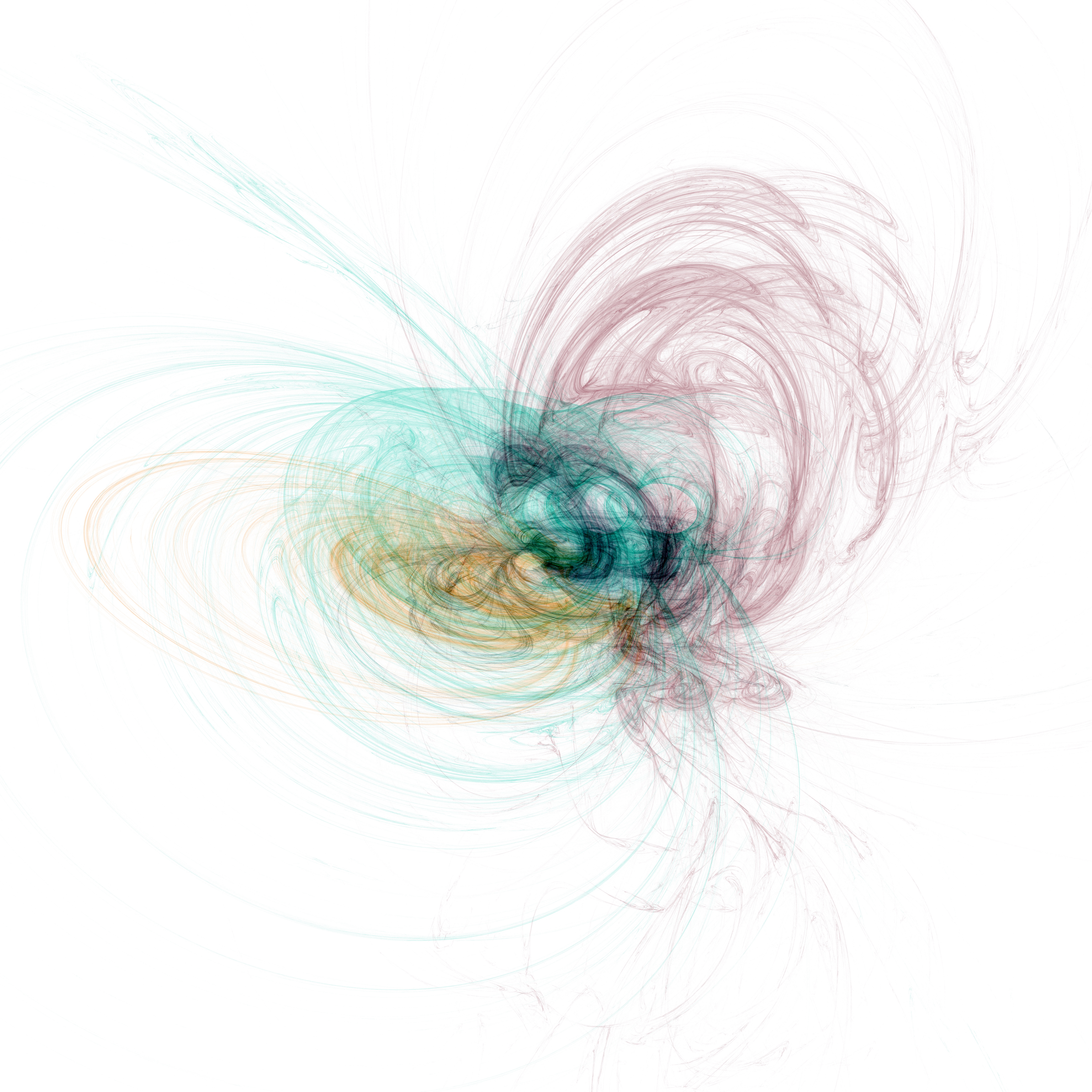
Fractal flames are a type of iterated function systems invented by Scott Draves in 1992. The fixed sets of fractal flames may be computed using the chaos game (as described in an earlier post), and the resulting histogram may be visualised as beautiful fractal-like images. If the histogram also has a dimension storing what function from the function system was used to get to a particular point, it may even be coloured.
There are a lot of software available to generate fractal flames, and I have built yet another one focussed on generating very high resolution images for printing. The image below has resolution 7087 x 7087 and been generated after about 4 hours of computation on a laptop. It is free to use under a Creative Commons BY-NC 4.0 license.
The Nørgård Palindrome is an ambient electronic music track released recently by Morten Bach and me. It is composed algorithmically and recorded live in studio using a lot of synthesizers. It is the second track of the album, the first being “Lorenz-6674089274190705457 (Seltsamer Attraktor)” which was described in another post.
The arpeggio-like tracks in The Nørgård Palindrome is created from an integer sequence first studied by the danish composer Per Nørgård in 1959 who called it an “infinite series”. It may be defined as
The sequence is interesting from a purely mathematical view point, which has been studied by several authors, for example by Au, Drexler-Lemire & Shallit (2017). Considering only the parity of the sequence yields the Thue-Morse sequence, which is a famous and well-studied sequence.
However, we will, as Per Nørgård, use the sequence to compose music. The sequence is most famously used in the symphony “Voyage into the Golden Screen”, where Per Nørgård mapped the first terms of the sequence to notes by picking a base note corresponding to 0 and then map an integer k to the note k semitones above the base note.
In The Nørgård Palindrome, we do the same, although we use a diatonic scale instead of a chromatic scale, and get the following notes when using a C-minor scale with 0 mapping to C:
It turns out that certain patterns are repeated throughout the sequence, although sometimes transposed, which makes the sequence very usable in music.
In the video below we play the first 144 notes slowly along while showing the progression of the corresponding sequence.
The first 144 notes of Nørgårds’ infinite series mapped to notes in a diatonic scale.
In The Nørgård Palindrome, we compute a large number of terms, allowing us to play the sequence very fast for a long time, and when done, we play the sequence backwards. This voice is played as a canon in two, and the places where the voices are in harmony or aligned emphasises the structure of the sequence.
The recurring theme is also composed from the sequence using a pentatonic scale and played slower.
The code use to generate the sequence and the MIDI-files used on the track is available on GitHub. The track is released as part of the album pieces of infinity 01 which is available on most streaming services, including Spotify and iTunes.
Lorenz-6674089274190705457 (Seltsamer Attraktor) is an ambient music track released by Morten Bach and me. It was composed algorithmically and recorded live in studio using a number of synthesizers. This post will describe how the track was composed.
The Lorenz system is a system of ordinary differential equations
where \sigma, \rho and \beta are positive real numbers. The system was first studied by Edward Lorenz and Helen Fetter as a simulation of atmospheric convection. It is known to behave chaotically for certain parameters since small changes in the starting point changes the future of a solution radically, an example of the so-called butterfly effect.
The differential equations above gives a formula for what direction a curve should move after it reaches a point (x,y,z) \in \mathbb{R}^3. As an example, for (1,1,1) we get the direction (0, \rho - 1, 1 - \beta).
In the composition of Lorenz-6674089274190705457 (Seltsamer Attraktor), we chose \sigma = 10, \rho = 28 and \beta = 2 and consider three curves with randomly chosen starting points. The number 6674089274190705457 is the seed of the pseudo-random number generator used to pick the starting points, so another seed would give other starting points and hence a different track.
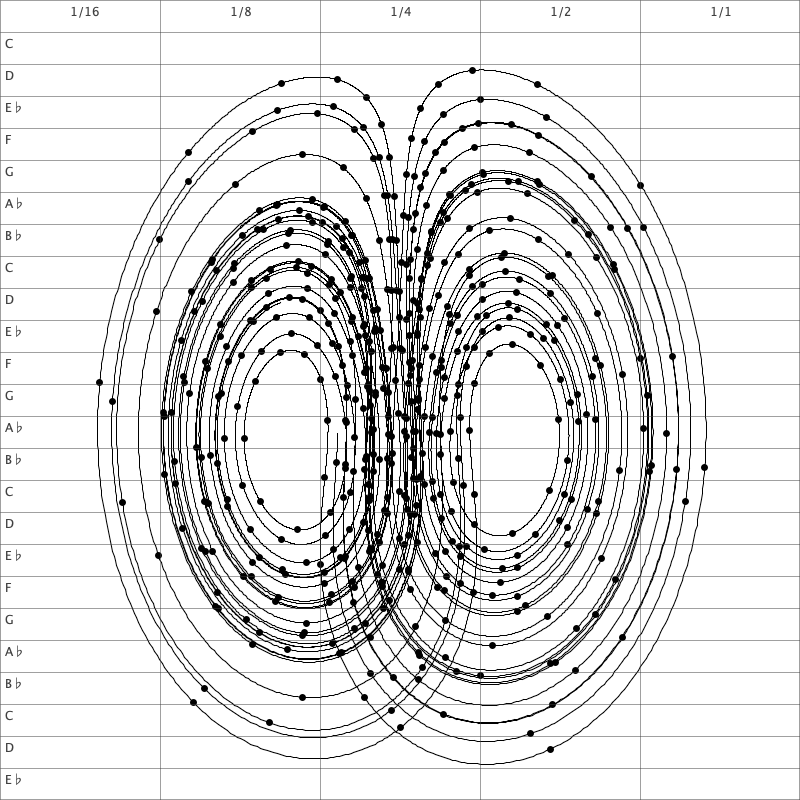
The curves are computed numerically. Above we show an example of a curve for t \in [0, 5]. The points corresponding to a discrete subset of the three curves we get from the given seed are mapped to notes. More precisely, we pick the points where t = 0.07k for k \in \mathbb{N}.
We consider the projection of curves to the (x,z)-plane. The part of this plane where the curve resides is divided into a grid as illustrated above. If the point to be mapped to a note is in the (i,j)‘th square, the note is chosen as the j‘th note in a predefined diatonic scale (in this case C-minor) with duration 2^{-i} time-units. The resulting track is saved as a MIDI-file.
The composition of the track is visualised in a video available on YouTube. Here, all three voices are shown as separate curves along with the actual track.
The Lorenz system and this mapping into musical notes was chosen to give an interesting, and somewhat linear (musically speaking) and continuously evolving dynamic. Using this mapping, the voices composed moves both fast and slow at different times. The continuity of the curves also ensures that the movement of each voice is linear (going either up or down continuously).
The track is available on most streaming services and music platforms, eg. Spotify or iTunes. The code used to generate the tracks is available on GitHub.
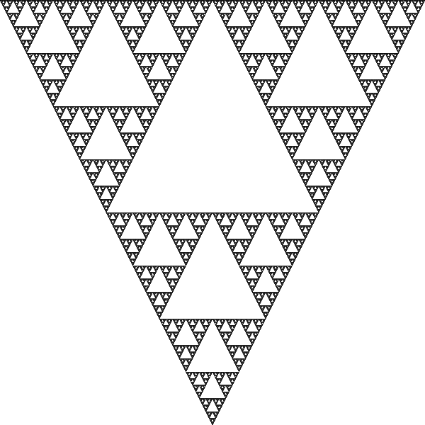
Many fractals may be described as the fixed set of an iterated function set (IFS). Perhaps most famously, the Sierpiński Triangle is such a fractal. Formally, an IFS is a set of maps on a metric space, eg. \mathbb{R}^n, which map points closer to each other.
Hutchinson proved in 1981 that an IFS has a unique compact fixed set S – a set where all points are mapped back into the set. Now, for some choices of IFS on the plane, the set S is very interesting and shows fractal properties. The Sierpiński Triangle is for example the fixed set of the following IFS:
A common way to visualise the fixed set of an IFS is by using the so-called Chaos game. Here, a point in the plane is picked at random. Then we apply one of the functions of the IFS, chosen at random, to the point. The result is another point in the plane which we again apply one of the function chosen at random on. At each step we plot the point, and we may continue for as long as we like and with as many initial points as we want.
The Sierpiński Triangle.
Another possible fractal which may be constructed as the fixed set of an IFS is the Barnsley Fern. Here the functions are (with points written as column vectors):
\begin{pmatrix} x \\ y \end{pmatrix} \mapsto \begin{pmatrix} 0 & 0 \\ 0 & 0.16 \end{pmatrix}\begin{pmatrix} x \\ y \end{pmatrix},
\begin{pmatrix} x \\ y \end{pmatrix} \mapsto \begin{pmatrix} 0.85 & 0.04 \\ -0.04 & 0.85 \end{pmatrix}\begin{pmatrix} x \\ y \end{pmatrix},
\begin{pmatrix} x \\ y \end{pmatrix} \mapsto \begin{pmatrix} 0.20 & -0.26 \\ 0.23 & 0.22 \end{pmatrix}\begin{pmatrix} x \\ y \end{pmatrix},
\begin{pmatrix} x \\ y \end{pmatrix} \mapsto \begin{pmatrix} -0.15 & 0.28 \\ 0.26 & 0.24 \end{pmatrix}\begin{pmatrix} x \\ y \end{pmatrix}.
Here, the the probability to pick the first map should be 1%, the second should be 85% and the remaining two should be 7% each. This will yield the picture below:
The Barnsley Fern.
A more complicated family of fractals representable by an IFS are the so-called fractal flames. For these fractals, the functions in their corresponding IFS’s are of the form P \circ V \circ T where P and T are affine linear transformations and V is a non-linear functions, a so-called variation.
A fractal flame.
Slowly transforming the parameters in the transformations of a fractal flame can be used to create movies.
Colouring the fractals may be done in different ways, the simplest being simply plotting each point while iterating in the chaos game. A slightly better way, which is used here, is the log-density method. Here the image to be rendered is divided into pixels, and the number of times each pixel is hit in the chaos game is saved. Now, the colour of a pixel is determined as the ratio \log n / \log m where n is the number of times the pixel was hit and m is the maximum number of times a pixel in the image has been hit.
The software used to generate the images in this post is available on GitHub.
I have recently read The Expected Goals Philosophy by James Tippett, where the idea behind “Expected goals” is explained very well. In The Expected Goals Philosophy, the probability that a given team will win based on their expected goals is computed by simulating the game many times, but it can actually be computed analytically which I will do here.
Also in The Expected Goals Philosophy, a phenomenon where a team creating a few good chances will win against a team creating many smaller chances even though the expected number of goals is exactly the same, is introduced and explained. Here I will give a different, and perhaps more rigorous explanation than the one given in the book to this curious phenomenon.
The distribution of xG
First, lets sum up the concept of expected goals: Given the shots a football team has during a match, each with some probability of ending up as a goal, the expected goals (xG) is the expected value of the total number of goals which equals the sum of the probabilities of each shot ending up in goal.
A shot with probability p of ending up in goal can be considered to be a Bernoulli random variable, so the expected goals of a team is the sum of many Bernoulli random variables, one for each shot. It follows that the expected goals of a team has a Poisson binomial distribution.
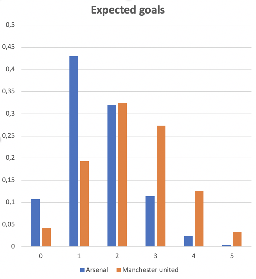
Consider the following example from The Expected Goals Philosophy. In 2019 Arsenal played Manchester United. The shots taken by each team and their estimated probabilities of ending up in goal are listed below:
Manchester United shots: (0.01, 0.02, 0.02, 0.02, 0.03, 0.05, 0.05, 0.05, 0.06, 0.22, 0.30, 0.43, 0.48, 0.63)
The expected value of a Poisson binomial distribution is the sum of the probabilities of each experiment (shot in this case), so calculating the expected goals for each team is simple: Arsenal has xG = 1.53 and Manchester United has xG = 2.37. But to consider the distribution of who will win the game, we need to consider the probability mass function of the expected goals which, as we saw, has a Poisson binomial distrbution.
The pmf of a Poisson binomial distributed random variable X with n parameters p_1, \ldots, p_n (shots with estimated xG’s in this case) may be calculated as follows: The probability that exactly k shots succeeds is equal to the sum of all possible combinations of k shots succeeding and the remaining n-k shots missed, e.g.
Here F_{k,n} is the set of all subsets of size k of \{1,\ldots,n\}. The pmf in this form is cumbersome to compute when the number of parameters (in this case the number of shots) increases. But luckily there are smarter ways to compute them, eg. a recursive method which is used in the code used to compute the actual distribution:
Now computing the probability of the possible outcomes of the game is straight-forward: For each possible number of goals Arsenal could have scored, we consider the probability that Manchester United has scored fewer, more or the same amount of goals. And since the event that Arsenal scores for example one goal and the event that Arsenal scores two goals are disjoint, the probabilities may be summed. Also, the expected goals of the two teams are assumed to be independent, so if we let A denote Arsenals xG and M denote Manchester Uniteds xG we for have:
Say we consider the event that Arsenal has scored two goals. Then the probability that they will win in this case is equal to the probability that Manchester United scored either a single goal or no goals. These probabilities are read from the above chart and added: 0.04 + 0.19 = 0.23.
This computation gives us the following probabilities for a win, draw or loose for Arsenal resp.: 0.18, 0.23, 0.59. These numbers are very close to the probabilities given in the The Expected Goals Philosophy where they were computed running 100.000 simulations.
Skewness of xG
In The Expected Goals Philosophy, a curious phenomenon is presented, namely that a team creating many small chances is more likely to loose to a team creating few large chances, even though the two teams’ expected number of goals are equal. In the book, the phenomenon is explained by the larger variance of the former teams xG, which is correct, but it is perhaps more precise to say, that it is due to the skewness of the distribution.
The example from the book is the case where one team, Team Coin, has four shots each with probability 1/2 of ending up in goal, and another team, Team Die Shots, has 12 shots each with probability 1/6 of ending up in goal. Since the probabilities for each shot ending up in goal are the same in the two cases, the xG for both teams are binomial distributed, which is somewhat simpler than the Poisson binomial distribution. A plot similar to the one above looks like this:
Note that Team Die’s is skewed to the right. In general, for binomial distributions, the distribution is symmetric if p = 0.5. But if p > 0.5, the distribution is skewed to the left (because the skewness is negative) and if p < 0.5, the distribution is skewed to the right (because the skewness is positive). In this case, Team Die’s distribution is skewed to the right so it has more of its mass to the left of the mean, meaning that the probability of scoring few goals is bigger than the probability of scoring more. Team Coin’s distribution, on the other hand, is completely symmetric (because the skewness is 0), meaning that the probability of scoring fewer goals than the mean is exactly the same as scoring more. Since the mean of the two are the same, the result is that Team Coin has a higher probability of ending up the winner.
The code for computing the distribution of the outcome of a football game based on the expected goals is available here.
Langton’s Ant is a simulation in two dimensions which has been proven to be a universal Turing machine – so it can in principal be used to compute anything computable by a computer.
The simulation consists of an infinite board of squares which can be either white or black. Now, an ant walks around the board. If the ant lands on a white square, it turns right, flips the color of the square and moves forward. one square If the square is black, the ant turns left, flips the color of the square and moves forward one square.
When visualised, the behaviour of this system changes over time from structured and simple to more chaotic. However, the system is completely deterministic, determined only by the starting state.
In the video above, a simulation with two ants runs over 500 steps and every time a square flips from black to white a note is played. The note to be played is determined as follows:
The board is divided into 7×7 sub-boards.
These squares are enumerated from the bottom left from 0 to 48.
When a square is flipped from black to white, the number assigned to the square determines the note as the number of semitones above A1.
Seven is chosen as the width of the sub-squares because it is the number of semitones in a fifth, so the ants moves either chromatically (horizontally) or in fifths (vertically). In the beginning, they are moving independently and very structured, but when their paths meet, a more complex, chaotic behaviour emerges.
Class inheritance and generics/templates makes it possible to write code with nice abstractions very similar to the abstractions used in math, particularly in abstract algebra, where a computation can be described for an entire class of algebraic structures sharing some similar properties (eg. groups and rings). This has been described nicely in the book “From Mathematics to Generic Programming” by Alexander A. Stepanov and Daniel E. Rose.
Inspired by this book, I have implemented a library for computations on abstract algebraic structures such as groups, rings and fields. The library is called Ruffini (named after the italian mathematician Paolo Ruffini) and is developed in Java using generics to achieve the same kind of abstraction as in abstract algebra, eg. that you do not specify what specific algebraic structure and elements are used, but only what abstract structure it has, eg. that it is a group or a ring.
Abstract algebraic structures are defined in Ruffini by a number of interfaces extending each other, each describing operations on elements of some set represented by a generic class E. The simplest such interface is a semigroup:
public interface Semigroup<E> {

  /**
   * Return the result of the product <i>ab</i> in this
   * semigroup.
   *
   * @param a An element <i>a</i> in this algebraic structure.
   * @param b Another element <i>b</i> in this algebraic
   *          structure.
   * @return The product of the two elements, <i>ab</i>.
   */
  public E multiply(E a, E b);

}
The semigroup is extended by a monoid interface which adds a getIdentity() method and by a group interface which adds an invert(E) method. Continuing like this, we end up with interfaces for more complicated structures like rings, fields and vector spaces.
Now, each of these interfaces describes functions that can be applied to a generic type E (eg. that given two instances of E, the multiply method above returns a new instance of type E). As in abstract algebra, these functions can be used to describe complicated computations without specifying exactly what algebraic structure is being used.
Ruffini currently implements a number of algorithms that is defined and described for the abstract structures, including the discrete Fourier transform, the Euclidean algorithm, computing Gröbner bases, the Gram-Schmidt process and Gaussian elimination. The abstraction makes it possible to write the algorithms only once in a clear, while still being usable on any of the algebraic structures defined in the library, such as integers, rational numbers, integers modulo n, finite fields, polynomial rings and matrix rings. Below is the code for the Gram-Schmidt process:
public List<V> apply(List<V> vectors) {
  List<V> U = new ArrayList<>();

  Projection<V, S> projection =
      new Projection<>(vectorSpace, innerProduct);

  for (V v : vectors) {
    for (V u : U) {
      V p = projection.apply(v, u);
      v = vectorSpace.subtract(v, p);
    }
    U.add(v);
  }
  return U;
}
Here V and S are the generic types for resp. the vectors and scalars of the underlying vector space, and Projection is a class defining projection given a specific vector space and an inner product.
Given a list of items each with a value and a weight, the Knapsack problem seeks to find the set of items with the largest combined value within a given weight limit. There are a nice dynamic programming solution which I decided to implement in a spread sheet. I used Google Sheets but the solution is exported as an excel-sheet.
The solution builds a Knapsack table for round 0,1,…,limit. In each round r the solution for the problem with limit r is constructed as a column in the table, so the table has to be as wide as the maximum limit. Once the table is built, the solution can be found using backtracking. This is all described pretty well on Wikipedia, https://en.wikipedia.org/wiki/Knapsack_problem#0/1_knapsack_problem.
The main challenge was to translate this algorithm from procedural pseudocode to a spreadsheet. Building the table is simple enough (once you learn the OFFSET command in Excel which allows you to add or subtract a variable number of rows and columns from a given position), but the backtracking was a bit more tricky.
Assuming that the weights are stored in column A from row 3 and the corresponding values are stored in column B, the table starts in column D. The round numbers are stored in row 1 from columnD. Row 2 are just 0’s and all other entries are (the one below is from D3):
The table stops after round 40, so we find the solution with weight at most 40.
The backtracking to find the actual solution after building the table is done in column AT and AU. In the first column, the number of weight spent after 40 rounds are calculated from bottom to top row using the formula (from AT3):
Given a set of linearly independent vectors, the Gram-Schmidt process produces a new set of vectors spanning the same subset, but the new set of vectors are now mutually orthogonal. The algorithm is usually stated as working over a vector space, but will in this post be altered to work over a module which is a vector space where the scalars are elements in a ring instead of a field. This could for instance be the case if we are given a set of integer vectors we wish to orthogonalise.
The original version can be described as follows: Given a set of vectors v_1, \ldots, v_n we define u_1 = v_1 and
for k = 2,3,\ldots,n. The projection operator is defined as
\text{proj}_u(v) = \frac{\langle u, v \rangle}{\langle u, u \rangle} u.
If we say that all v_i have integer entries, we see that u_i must have rational entries, and simply scaling each vector with a multiple of all the denominators of the entries will give a vector parallel to the original vector but with integer entries. But what if we are interested in an algorithm that can only represent integers?
The algorithm is presented below. Note that the algorithm works over any module with inner product (aka a Hilbert Module).
# Given: Set of vectors V.
# Returns: A set of mutually orthogonal vectors spanning
# the same subspace as the vectors in V.

U := Ø
k := 1

while V ≠ Ø do
  poll vector v from V
  w := kv

  for (u,m) in U do
    w -= m〈v,u〉u

  # Optional: Divide all entries in w by gcd of entries

  if V ≠ Ø do
    n :=〈w,w〉
    for (u,m) in U do
      m *= n
    Put (w,k) in U
    k *= n
  else do
    # No more iterations after this one
    Put (w,k) in U

return first coordinates of elements in U
When used on integers, the entries in the vectors grow very fast, but this may be avoided by dividing w by the greatest common divisor of the entries.