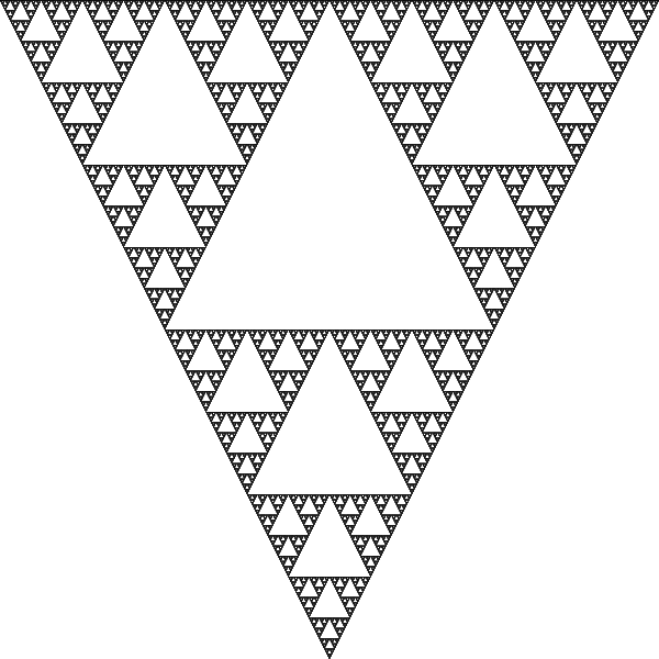
Many fractals may be described as the fixed set of an iterated function set (IFS). Perhaps most famously, the Sierpiński Triangle is such a fractal. Formally, an IFS is a set of maps on a metric space, eg. \mathbb{R}^n, which map points closer to each other.
Hutchinson proved in 1981 that an IFS has a unique compact fixed set S – a set where all points are mapped back into the set. Now, for some choices of IFS on the plane, the set S is very interesting and shows fractal properties. The Sierpiński Triangle is for example the fixed set of the following IFS:
A common way to visualise the fixed set of an IFS is by using the so-called Chaos game. Here, a point in the plane is picked at random. Then we apply one of the functions of the IFS, chosen at random, to the point. The result is another point in the plane which we again apply one of the function chosen at random on. At each step we plot the point, and we may continue for as long as we like and with as many initial points as we want.
Another possible fractal which may be constructed as the fixed set of an IFS is the Barnsley Fern. Here the functions are (with points written as column vectors):
Here, the the probability to pick the first map should be 1%, the second should be 85% and the remaining two should be 7% each. This will yield the picture below:

A more complicated family of fractals representable by an IFS are the so-called fractal flames. For these fractals, the functions in their corresponding IFS’s are of the form P \circ V \circ T where P and T are affine linear transformations and V is a non-linear functions, a so-called variation.

Slowly transforming the parameters in the transformations of a fractal flame can be used to create movies.
Colouring the fractals may be done in different ways, the simplest being simply plotting each point while iterating in the chaos game. A slightly better way, which is used here, is the log-density method. Here the image to be rendered is divided into pixels, and the number of times each pixel is hit in the chaos game is saved. Now, the colour of a pixel is determined as the ratio \log n / \log m where n is the number of times the pixel was hit and m is the maximum number of times a pixel in the image has been hit.
The software used to generate the images in this post is available on GitHub.